19 July 2021 / DEEPLEARNING

Deep Learning from Scratch - Neural Network

Activation Function

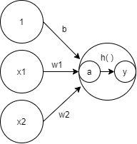
입력 신호의 총합을 출력 신호로 변환하는 함수를 활성화 함수(activation function)이라고 한다. 신호의 총합을 계산하고 활성화 함수에 입력해 결과를 내는 2단계로 나눠보면

$a = b + w_{1}x_{1} + w_{2}x_{2}$ $ y = h(a)$

activation_function

import numpy as np
import matplotlib.pyplot as plt
import warnings
warnings.filterwarnings('ignore')

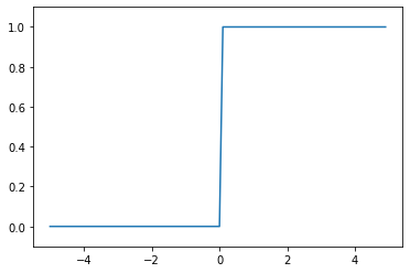
Step Function

def step_function(x):
    y = x > 0
    return y.astype(np.int)

x = np.array([-1.0, 1.0, 2.0])

step_function(x)

array([0, 1, 1])

x = np.arange(-5.0, 5.0, 0.1)
y = step_function(x)
plt.plot(x,y)
plt.ylim(-0.1, 1.1)
plt.show()

png

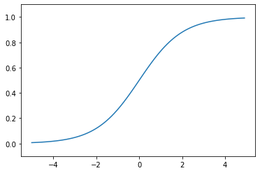
Sigmoid Function

$h(x) = \frac{1}{1+e^{-x}}$

def sigmoid(x):
    return 1 / (1 + np.exp(-x))

x = np.array([-1.0, 1.0, 2.0])
sigmoid(x)

array([0.26894142, 0.73105858, 0.88079708])

x = np.arange(-5.0, 5.0, 0.1)
y = sigmoid(x)
plt.plot(x, y)
plt.ylim(-0.1, 1.1)
plt.show()

png

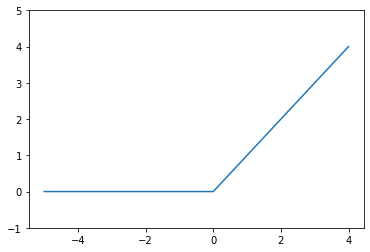
ReLU

def relu(x):
    return np.maximum(0, x)

x = [-5, 0, 4]
y = relu(x)
plt.plot(x, y)
plt.ylim(-1, 5)
plt.show()

png

신경망에서의 행렬 곱

X = np.array([1, 2])
print(X, X.shape)

[1 2] (2,)

W = np.array([[1,3,5], [2,4,6]])
print(W, W.shape)

[[1 3 5]
 [2 4 6]] (2, 3)

Y = np.dot(X, W)
print(Y, Y.shape)

[ 5 11 17] (3,)

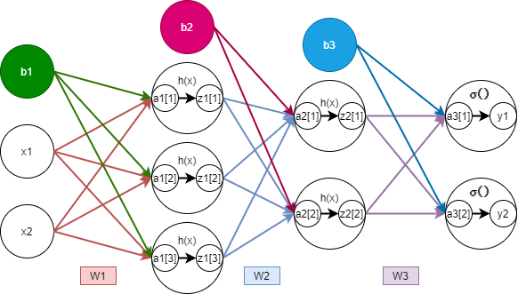
3층 신경망 구현하기

3layer

def identity_function(x):
    return x

def init_network():
    network = {}
    network['W1'] = np.array([[.1, .3, .5], [.2, .4, .6]])
    network['b1'] = np.array([.1, .2, .3])
    network['W2'] = np.array([[.1, .4], [.2, .5], [.3, .6]])
    network['b2'] = np.array([.1, .2])
    network['W3'] = np.array([[.1, .3], [.2, .4]])
    network['b3'] = np.array([.1, .2])
    
    return network

def forward(network, x):
    W1, W2, W3 = network['W1'], network['W2'], network['W3']
    b1, b2, b3 = network['b1'], network['b2'], network['b3']
    
    a1 = np.dot(x, W1) + b1
    z1 = sigmoid(a1)
    a2 = np.dot(z1, W2) + b2
    z2 = sigmoid(a2)
    a3 = np.dot(z2, W3) + b3
    y = identity_function(a3)
    
    return y

network = init_network()
x = np.array([1.0, 0.5])
y = forward(network, x)
print(y)

[0.31682708 0.69627909]

출력층 설계하기

Identity Function

입력 신호가 그대로 출력 신호가 된다.

Softmax Function

softmax

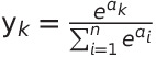
$n$은 출력층의 뉴런 수, $y_{k}$는 그중 $k$번째 출력임을 뜻한다. softmax 함수의 분자는 입력 신호 $a_{k}$의 지수 함수, 분모는 모든 입력 신호의 지수 함수의 합으로 구성된다.

a = np.array([.3, 2.9, 4.0])
exp_a = np.exp(a)
print(exp_a)

[ 1.34985881 18.17414537 54.59815003]

sum_exp_a = np.sum(exp_a)
print(sum_exp_a)

74.1221542101633

y = exp_a / sum_exp_a
print(y)

[0.01821127 0.24519181 0.73659691]

def softmax(a):
    exp_a = np.exp(a)
    sum_exp_a = np.sum(exp_a)
    y = exp_a / sum_exp_a
    
    return y

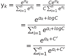
주의점

softmax 함수는 지수 함수를 사용하기 때문에 큰 값은 inf가 되어 돌아오고 오버플로 문제가 발생할 수 있다. softmax 함수를 개선해보면, softmax revise

a = np.array([1010, 1000, 990])
np.exp(a) / np.sum(np.exp(a))

array([nan, nan, nan])

c = np.max(a)
a - c

array([  0, -10, -20])

np.exp(a-c) / np.sum(np.exp(a - c))

array([9.99954600e-01, 4.53978686e-05, 2.06106005e-09])

단순히 softmax로 계산하게 되면 nan이 출력된다. 하지만 입력 신호 중 최댓값을 빼주면 올바르게 계산할 수 있으며 이를 구현하면

def softmax(a):
    c = np.max(a)
    exp_a = np.exp(a - c)
    sum_exp_a = np.sum(exp_a)
    y = exp_a / sum_exp_a
    
    return y

Softmax Function 특징

a = np.array([.3, 2.9, 4.0])
y = softmax(a)
print(y, np.sum(y))

[0.01821127 0.24519181 0.73659691] 1.0

Softmax function은 0에서 1.0 사이의 실수이다. 또한 총합은 1이 된다. 이 성질 덕분에 출력을 확률로 해석할 수 있다. 또한 softmax function을 적용해도 출력이 가장 큰 뉴런의 위치는 달라지지 않는다. 결과적으로 신경망으로 분류할때는 출력층의 softmax function을 생략해도 된다.

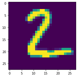
MNIST

import tensorflow as tf
import matplotlib.pyplot as plt
import pickle
import time

def plot_img(img):
    img = np.uint8(img)
    plt.imshow(img.reshape(28, 28))

def get_data():
    mnist = tf.keras.datasets.mnist
    (x_train, y_train), (x_test, y_test) = mnist.load_data()
    x_train = x_train.reshape(-1, 784)
    x_test = x_test.reshape(-1, 784)
    
    return x_test, y_test

img, _ = get_data()

plot_img(img[1])

png

def init_network():
    with open('sample_weight.pkl', 'rb') as f:
        network = pickle.load(f)
    return network

def predict(network, x):
    W1, W2, W3 = network['W1'], network['W2'], network['W3']
    b1, b2, b3 = network['b1'], network['b2'], network['b3']

    a1 = np.dot(x, W1) + b1
    z1 = sigmoid(a1)
    a2 = np.dot(z1, W2) + b2
    z2 = sigmoid(a2)
    a3 = np.dot(z2, W3) + b3
    y = softmax(a3)

    return y

network = init_network()

x, t = x_test, y_test

start_time = time.time()
accuracy_cnt = 0
for i in range(len(x)):
    y = predict(network, x[i])
    p = np.argmax(y)
    if p == t[i]:
        accuracy_cnt += 1

end_time = time.time()
no_batch_time = end_time - start_time
print('Accuracy: '+str(float(accuracy_cnt) / len(x)), f', time elapsed : {end_time - start_time}')

Accuracy: 0.9207 , time elapsed : 1.0659980773925781

Batch 처리

x, _ = get_data()

network = init_network()

W1, W2, W3 = network['W1'], network['W2'], network['W3']
x.shape

(10000, 784)

print(x[0].shape, W1.shape, W2.shape, W3.shape)

(784,) (784, 50) (50, 100) (100, 10)

x, t = get_data()
network = init_network()

batch_size = 100

accuracy_cnt = 0

start_time = time.time()
for i in range(0, len(x), batch_size):
    x_batch = x[i:i+batch_size]
    y_batch = predict(network, x_batch)
    p = np.argmax(y_batch, axis=1)
    accuracy_cnt += np.sum(p == t[i:i+batch_size])

end_time = time.time()
batch_time = end_time - start_time
print('Accuracy: '+str(float(accuracy_cnt) / len(x)), f', time elapsed : {end_time - start_time}')
print(f'Time saved {np.round((no_batch_time - batch_time), 6)} seconde')

Accuracy: 0.9207 , time elapsed : 0.06101250648498535
Time saved 1.004986 seconde

Keras

from tensorflow.keras.layers import Dense, Input
from tensorflow.keras.models import Model
from tensorflow.keras.utils import to_categorical

x_train, y_train, x_test, y_test = get_data()

x_train.shape

(60000, 784)

y_train_categorical = to_categorical(y_train)

inputs = Input(shape=(784, ))
d = Dense(50, activation ='sigmoid')(inputs)
d = Dense(100, activation='sigmoid')(d)
d = Dense(10, activation='softmax')(d)
model = Model(inputs, d)

model.summary()

Model: "functional_10"
_________________________________________________________________
Layer (type)                 Output Shape              Param #   
=================================================================
input_7 (InputLayer)         [(None, 784)]             0         
_________________________________________________________________
dense_16 (Dense)             (None, 50)                39250     
_________________________________________________________________
dense_17 (Dense)             (None, 100)               5100      
_________________________________________________________________
dense_18 (Dense)             (None, 10)                1010      
=================================================================
Total params: 45,360
Trainable params: 45,360
Non-trainable params: 0
_________________________________________________________________

model.compile(loss='mse', optimizer='adam')

start_time = time.time()
hist = model.fit(x_train, y_train_categorical, epochs = 20)
end_time = time.time()
print(f'time elapsed {end_time - start_time}')

Epoch 1/20
1875/1875 [==============================] - 2s 809us/step - loss: 0.0317
Epoch 2/20
1875/1875 [==============================] - 2s 812us/step - loss: 0.0202
Epoch 3/20
1875/1875 [==============================] - 2s 820us/step - loss: 0.0187
Epoch 4/20
1875/1875 [==============================] - 2s 823us/step - loss: 0.0177
Epoch 5/20
1875/1875 [==============================] - 2s 814us/step - loss: 0.0177
Epoch 6/20
1875/1875 [==============================] - 2s 829us/step - loss: 0.0173
Epoch 7/20
1875/1875 [==============================] - 2s 826us/step - loss: 0.0166
Epoch 8/20
1875/1875 [==============================] - 2s 819us/step - loss: 0.0159
Epoch 9/20
1875/1875 [==============================] - 2s 817us/step - loss: 0.0148
Epoch 10/20
1875/1875 [==============================] - 2s 823us/step - loss: 0.0152
Epoch 11/20
1875/1875 [==============================] - 2s 821us/step - loss: 0.0143
Epoch 12/20
1875/1875 [==============================] - 2s 841us/step - loss: 0.0142
Epoch 13/20
1875/1875 [==============================] - 2s 823us/step - loss: 0.0137
Epoch 14/20
1875/1875 [==============================] - 2s 844us/step - loss: 0.0133
Epoch 15/20
1875/1875 [==============================] - 2s 858us/step - loss: 0.0128
Epoch 16/20
1875/1875 [==============================] - 2s 854us/step - loss: 0.0128
Epoch 17/20
1875/1875 [==============================] - 2s 833us/step - loss: 0.0126
Epoch 18/20
1875/1875 [==============================] - 2s 826us/step - loss: 0.0129
Epoch 19/20
1875/1875 [==============================] - 2s 819us/step - loss: 0.0123
Epoch 20/20
1875/1875 [==============================] - 2s 830us/step - loss: 0.0122
time elapsed 31.24882459640503

predict = model.predict(x_test)

predicted_label = predict.argmax(axis=1)

cnt = 0
for i in range(len(predicted_label)):
    if (predicted_label[i] == y_test[i]):
        cnt += 1

print(f'Accuracy : {cnt / len(predicted_label) * 100}')

Accuracy : 91.57

Torch

import torch
import torch.nn as nn
import torch.nn.functional as F
import torch.optim as optim
from torchvision import datasets, transforms

class dnn(nn.Module):
    
    def __init__(self):
        super(dnn, self).__init__()
        self.d1 = nn.Linear(784, 50)
        self.d2 = nn.Linear(50, 100)
        self.d3 = nn.Linear(100, 10)
        
    def forward(self, x):
        x = x.float()
        h1 = F.sigmoid(self.d1(x.view(-1, 784)))
        h2 = F.sigmoid(self.d2(h1))
        
        return F.softmax(h2, dim=1)

transform = transforms.Compose([transforms.ToTensor(), transforms.Normalize((0.1307, ), (0.3081, ))])
train_loader = torch.utils.data.DataLoader(datasets.MNIST('../data', train=True, download=True, transform=transform))
test_loader = torch.utils.data.DataLoader(datasets.MNIST('../data', train=False, download=True, transform=transform))

model = dnn()

optimizer = optim.Adam(model.parameters())
no_cuda = True
use_cuda = not no_cuda and torch.cuda.is_available()
device = torch.device("cuda" if use_cuda else "cpu")

batch_size = 64
interval = 20000
epoch = 10

def train(interval, model, device, train_loader, optimizer, epoch):
    model.train()
    for batch_idx, (data, target) in enumerate(train_loader):
        data, target = data.to(device), target.to(device)
        optimizer.zero_grad()
        output = model(data)
        loss = F.nll_loss(output, target)
        loss.backward()
        optimizer.step()
        if batch_idx % interval == 0:
            print('Train Epoch: {} [{}/{} ({:.0f}%)]\tLoss: {:.6f}'.format(epoch, batch_idx * len(data), len(train_loader.dataset),100. * batch_idx / len(train_loader), loss.item()))
            
def test(interval, model, device, test_loader):
    model.eval()
    test_loss = 0
    correct = 0
    with torch.no_grad():
        for data, target in test_loader:
            data, target = data.to(device), target.to(device)
            output = model(data)
            test_loss += F.nll_loss(output, target, reduction='sum').item()
            pred = output.argmax(dim=1, keepdim=True)
            correct += pred.eq(target.view_as(pred)).sum().item()
            
    test_loss /= len(test_loader.dataset)
    
    print('\nTest set: Average loss: {:.4f}, Accuracy: {}/{} ({:.0f}%)\n'.format(test_loss, correct, len(test_loader.dataset),100. * correct / len(test_loader.dataset)))

for epoch in range(1, 11):
    train(interval, model, device, train_loader, optimizer, epoch)
    test(interval, model, device, test_loader)

Train Epoch: 1 [0/60000 (0%)]	Loss: -0.008938
Train Epoch: 1 [20000/60000 (33%)]	Loss: -0.025429
Train Epoch: 1 [40000/60000 (67%)]	Loss: -0.025821

Test set: Average loss: -0.0254, Accuracy: 1034/10000 (10%)

Train Epoch: 2 [0/60000 (0%)]	Loss: -0.025665
Train Epoch: 2 [20000/60000 (33%)]	Loss: -0.026105
Train Epoch: 2 [40000/60000 (67%)]	Loss: -0.025847

Test set: Average loss: -0.0257, Accuracy: 8315/10000 (83%)

Train Epoch: 3 [0/60000 (0%)]	Loss: -0.025708
Train Epoch: 3 [20000/60000 (33%)]	Loss: -0.026541
Train Epoch: 3 [40000/60000 (67%)]	Loss: -0.026278

Test set: Average loss: -0.0259, Accuracy: 8550/10000 (86%)

Train Epoch: 4 [0/60000 (0%)]	Loss: -0.026034
Train Epoch: 4 [20000/60000 (33%)]	Loss: -0.026690
Train Epoch: 4 [40000/60000 (67%)]	Loss: -0.026271

Test set: Average loss: -0.0259, Accuracy: 8810/10000 (88%)

Train Epoch: 5 [0/60000 (0%)]	Loss: -0.026035
Train Epoch: 5 [20000/60000 (33%)]	Loss: -0.026684
Train Epoch: 5 [40000/60000 (67%)]	Loss: -0.026274

Test set: Average loss: -0.0259, Accuracy: 8695/10000 (87%)

Train Epoch: 6 [0/60000 (0%)]	Loss: -0.026662
Train Epoch: 6 [20000/60000 (33%)]	Loss: -0.026507
Train Epoch: 6 [40000/60000 (67%)]	Loss: -0.026301

Test set: Average loss: -0.0260, Accuracy: 8914/10000 (89%)

Train Epoch: 7 [0/60000 (0%)]	Loss: -0.026341
Train Epoch: 7 [20000/60000 (33%)]	Loss: -0.026646
Train Epoch: 7 [40000/60000 (67%)]	Loss: -0.026506

Test set: Average loss: -0.0260, Accuracy: 8853/10000 (89%)

Train Epoch: 8 [0/60000 (0%)]	Loss: -0.026542
Train Epoch: 8 [20000/60000 (33%)]	Loss: -0.026723
Train Epoch: 8 [40000/60000 (67%)]	Loss: -0.026484

Test set: Average loss: -0.0260, Accuracy: 8787/10000 (88%)

Train Epoch: 9 [0/60000 (0%)]	Loss: -0.026377
Train Epoch: 9 [20000/60000 (33%)]	Loss: -0.026722
Train Epoch: 9 [40000/60000 (67%)]	Loss: -0.026350

Test set: Average loss: -0.0260, Accuracy: 8703/10000 (87%)

Train Epoch: 10 [0/60000 (0%)]	Loss: -0.026281
Train Epoch: 10 [20000/60000 (33%)]	Loss: -0.026713
Train Epoch: 10 [40000/60000 (67%)]	Loss: -0.026708

Test set: Average loss: -0.0260, Accuracy: 8549/10000 (85%)

참고 : 사이토 고키, 『DeepLearning from Scratch』, 한빛미디어(2020), p63-105