Time Series Analysis - Multivariage Time Series with LSTM & RNNs
Multivariate Time Series
import pandas as pd
import numpy as np
%matplotlib inline
import matplotlib.pyplot as plt
df = pd.read_csv('MultiVariate-RNN-with-TensorFlow-and-Keras-master/DATA/energydata_complete.csv', index_col='date',infer_datetime_format=True)
df.head()
| Appliances | lights | T1 | RH_1 | T2 | RH_2 | T3 | RH_3 | T4 | RH_4 | ... | T9 | RH_9 | T_out | Press_mm_hg | RH_out | Windspeed | Visibility | Tdewpoint | rv1 | rv2 | |
|---|---|---|---|---|---|---|---|---|---|---|---|---|---|---|---|---|---|---|---|---|---|
| date | |||||||||||||||||||||
| 2016-01-11 17:00:00 | 60 | 30 | 19.89 | 47.596667 | 19.2 | 44.790000 | 19.79 | 44.730000 | 19.000000 | 45.566667 | ... | 17.033333 | 45.53 | 6.600000 | 733.5 | 92.0 | 7.000000 | 63.000000 | 5.3 | 13.275433 | 13.275433 |
| 2016-01-11 17:10:00 | 60 | 30 | 19.89 | 46.693333 | 19.2 | 44.722500 | 19.79 | 44.790000 | 19.000000 | 45.992500 | ... | 17.066667 | 45.56 | 6.483333 | 733.6 | 92.0 | 6.666667 | 59.166667 | 5.2 | 18.606195 | 18.606195 |
| 2016-01-11 17:20:00 | 50 | 30 | 19.89 | 46.300000 | 19.2 | 44.626667 | 19.79 | 44.933333 | 18.926667 | 45.890000 | ... | 17.000000 | 45.50 | 6.366667 | 733.7 | 92.0 | 6.333333 | 55.333333 | 5.1 | 28.642668 | 28.642668 |
| 2016-01-11 17:30:00 | 50 | 40 | 19.89 | 46.066667 | 19.2 | 44.590000 | 19.79 | 45.000000 | 18.890000 | 45.723333 | ... | 17.000000 | 45.40 | 6.250000 | 733.8 | 92.0 | 6.000000 | 51.500000 | 5.0 | 45.410389 | 45.410389 |
| 2016-01-11 17:40:00 | 60 | 40 | 19.89 | 46.333333 | 19.2 | 44.530000 | 19.79 | 45.000000 | 18.890000 | 45.530000 | ... | 17.000000 | 45.40 | 6.133333 | 733.9 | 92.0 | 5.666667 | 47.666667 | 4.9 | 10.084097 | 10.084097 |
5 rows × 28 columns
df.info()
<class 'pandas.core.frame.DataFrame'>
Index: 19735 entries, 2016-01-11 17:00:00 to 2016-05-27 18:00:00
Data columns (total 28 columns):
 #   Column       Non-Null Count  Dtype
---  ------       --------------  -----
 0   Appliances   19735 non-null  int64
 1   lights       19735 non-null  int64
 2   T1           19735 non-null  float64
 3   RH_1         19735 non-null  float64
 4   T2           19735 non-null  float64
 5   RH_2         19735 non-null  float64
 6   T3           19735 non-null  float64
 7   RH_3         19735 non-null  float64
 8   T4           19735 non-null  float64
 9   RH_4         19735 non-null  float64
 10  T5           19735 non-null  float64
 11  RH_5         19735 non-null  float64
 12  T6           19735 non-null  float64
 13  RH_6         19735 non-null  float64
 14  T7           19735 non-null  float64
 15  RH_7         19735 non-null  float64
 16  T8           19735 non-null  float64
 17  RH_8         19735 non-null  float64
 18  T9           19735 non-null  float64
 19  RH_9         19735 non-null  float64
 20  T_out        19735 non-null  float64
 21  Press_mm_hg  19735 non-null  float64
 22  RH_out       19735 non-null  float64
 23  Windspeed    19735 non-null  float64
 24  Visibility   19735 non-null  float64
 25  Tdewpoint    19735 non-null  float64
 26  rv1          19735 non-null  float64
 27  rv2          19735 non-null  float64
dtypes: float64(26), int64(2)
memory usage: 4.4+ MB
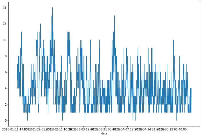
df['Windspeed'].plot(figsize=(12,8))
<AxesSubplot:xlabel='date'>
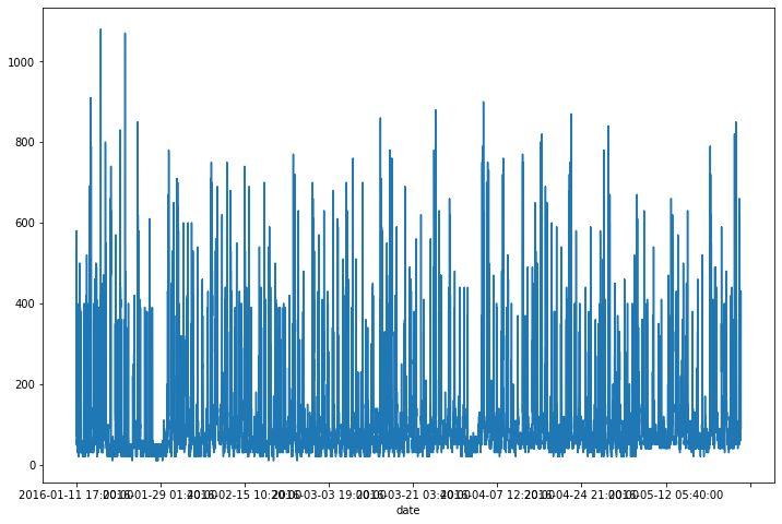
df['Appliances'].plot(figsize=(12,8))
<AxesSubplot:xlabel='date'>
Train Test Split
len(df)
19735
df.loc['2016-05-01':]
| Appliances | lights | T1 | RH_1 | T2 | RH_2 | T3 | RH_3 | T4 | RH_4 | ... | T9 | RH_9 | T_out | Press_mm_hg | RH_out | Windspeed | Visibility | Tdewpoint | rv1 | rv2 | |
|---|---|---|---|---|---|---|---|---|---|---|---|---|---|---|---|---|---|---|---|---|---|
| date | |||||||||||||||||||||
| 2016-05-01 00:00:00 | 50 | 0 | 21.200000 | 38.200000 | 18.390000 | 41.400000 | 23.200000 | 36.400000 | 19.73 | 37.730000 | ... | 19.166667 | 38.200000 | 4.300000 | 763.700000 | 86.000000 | 2.000000 | 40.000000 | 2.200000 | 15.310003 | 15.310003 |
| 2016-05-01 00:10:00 | 60 | 0 | 21.150000 | 38.172500 | 18.390000 | 41.500000 | 23.133333 | 36.466667 | 19.70 | 37.663333 | ... | 19.133333 | 38.290000 | 4.283333 | 763.716667 | 86.333333 | 2.166667 | 38.166667 | 2.216667 | 11.240067 | 11.240067 |
| 2016-05-01 00:20:00 | 50 | 0 | 21.133333 | 38.090000 | 18.323333 | 41.500000 | 23.200000 | 36.500000 | 19.70 | 37.590000 | ... | 19.133333 | 38.363333 | 4.266667 | 763.733333 | 86.666667 | 2.333333 | 36.333333 | 2.233333 | 21.808814 | 21.808814 |
| 2016-05-01 00:30:00 | 50 | 0 | 21.100000 | 38.090000 | 18.290000 | 41.500000 | 23.200000 | 36.500000 | 19.70 | 37.500000 | ... | 19.166667 | 38.500000 | 4.250000 | 763.750000 | 87.000000 | 2.500000 | 34.500000 | 2.250000 | 47.000534 | 47.000534 |
| 2016-05-01 00:40:00 | 60 | 0 | 21.100000 | 38.030000 | 18.290000 | 41.560000 | 23.200000 | 36.500000 | 19.70 | 37.500000 | ... | 19.166667 | 38.633333 | 4.233333 | 763.766667 | 87.333333 | 2.666667 | 32.666667 | 2.266667 | 8.059441 | 8.059441 |
| ... | ... | ... | ... | ... | ... | ... | ... | ... | ... | ... | ... | ... | ... | ... | ... | ... | ... | ... | ... | ... | ... |
| 2016-05-27 17:20:00 | 100 | 0 | 25.566667 | 46.560000 | 25.890000 | 42.025714 | 27.200000 | 41.163333 | 24.70 | 45.590000 | ... | 23.200000 | 46.790000 | 22.733333 | 755.200000 | 55.666667 | 3.333333 | 23.666667 | 13.333333 | 43.096812 | 43.096812 |
| 2016-05-27 17:30:00 | 90 | 0 | 25.500000 | 46.500000 | 25.754000 | 42.080000 | 27.133333 | 41.223333 | 24.70 | 45.590000 | ... | 23.200000 | 46.790000 | 22.600000 | 755.200000 | 56.000000 | 3.500000 | 24.500000 | 13.300000 | 49.282940 | 49.282940 |
| 2016-05-27 17:40:00 | 270 | 10 | 25.500000 | 46.596667 | 25.628571 | 42.768571 | 27.050000 | 41.690000 | 24.70 | 45.730000 | ... | 23.200000 | 46.790000 | 22.466667 | 755.200000 | 56.333333 | 3.666667 | 25.333333 | 13.266667 | 29.199117 | 29.199117 |
| 2016-05-27 17:50:00 | 420 | 10 | 25.500000 | 46.990000 | 25.414000 | 43.036000 | 26.890000 | 41.290000 | 24.70 | 45.790000 | ... | 23.200000 | 46.817500 | 22.333333 | 755.200000 | 56.666667 | 3.833333 | 26.166667 | 13.233333 | 6.322784 | 6.322784 |
| 2016-05-27 18:00:00 | 430 | 10 | 25.500000 | 46.600000 | 25.264286 | 42.971429 | 26.823333 | 41.156667 | 24.70 | 45.963333 | ... | 23.200000 | 46.845000 | 22.200000 | 755.200000 | 57.000000 | 4.000000 | 27.000000 | 13.200000 | 34.118851 | 34.118851 |
3853 rows × 28 columns
df = df.loc['2016-05-01':]
df = df.round(2)
df
| Appliances | lights | T1 | RH_1 | T2 | RH_2 | T3 | RH_3 | T4 | RH_4 | ... | T9 | RH_9 | T_out | Press_mm_hg | RH_out | Windspeed | Visibility | Tdewpoint | rv1 | rv2 | |
|---|---|---|---|---|---|---|---|---|---|---|---|---|---|---|---|---|---|---|---|---|---|
| date | |||||||||||||||||||||
| 2016-05-01 00:00:00 | 50 | 0 | 21.20 | 38.20 | 18.39 | 41.40 | 23.20 | 36.40 | 19.73 | 37.73 | ... | 19.17 | 38.20 | 4.30 | 763.70 | 86.00 | 2.00 | 40.00 | 2.20 | 15.31 | 15.31 |
| 2016-05-01 00:10:00 | 60 | 0 | 21.15 | 38.17 | 18.39 | 41.50 | 23.13 | 36.47 | 19.70 | 37.66 | ... | 19.13 | 38.29 | 4.28 | 763.72 | 86.33 | 2.17 | 38.17 | 2.22 | 11.24 | 11.24 |
| 2016-05-01 00:20:00 | 50 | 0 | 21.13 | 38.09 | 18.32 | 41.50 | 23.20 | 36.50 | 19.70 | 37.59 | ... | 19.13 | 38.36 | 4.27 | 763.73 | 86.67 | 2.33 | 36.33 | 2.23 | 21.81 | 21.81 |
| 2016-05-01 00:30:00 | 50 | 0 | 21.10 | 38.09 | 18.29 | 41.50 | 23.20 | 36.50 | 19.70 | 37.50 | ... | 19.17 | 38.50 | 4.25 | 763.75 | 87.00 | 2.50 | 34.50 | 2.25 | 47.00 | 47.00 |
| 2016-05-01 00:40:00 | 60 | 0 | 21.10 | 38.03 | 18.29 | 41.56 | 23.20 | 36.50 | 19.70 | 37.50 | ... | 19.17 | 38.63 | 4.23 | 763.77 | 87.33 | 2.67 | 32.67 | 2.27 | 8.06 | 8.06 |
| ... | ... | ... | ... | ... | ... | ... | ... | ... | ... | ... | ... | ... | ... | ... | ... | ... | ... | ... | ... | ... | ... |
| 2016-05-27 17:20:00 | 100 | 0 | 25.57 | 46.56 | 25.89 | 42.03 | 27.20 | 41.16 | 24.70 | 45.59 | ... | 23.20 | 46.79 | 22.73 | 755.20 | 55.67 | 3.33 | 23.67 | 13.33 | 43.10 | 43.10 |
| 2016-05-27 17:30:00 | 90 | 0 | 25.50 | 46.50 | 25.75 | 42.08 | 27.13 | 41.22 | 24.70 | 45.59 | ... | 23.20 | 46.79 | 22.60 | 755.20 | 56.00 | 3.50 | 24.50 | 13.30 | 49.28 | 49.28 |
| 2016-05-27 17:40:00 | 270 | 10 | 25.50 | 46.60 | 25.63 | 42.77 | 27.05 | 41.69 | 24.70 | 45.73 | ... | 23.20 | 46.79 | 22.47 | 755.20 | 56.33 | 3.67 | 25.33 | 13.27 | 29.20 | 29.20 |
| 2016-05-27 17:50:00 | 420 | 10 | 25.50 | 46.99 | 25.41 | 43.04 | 26.89 | 41.29 | 24.70 | 45.79 | ... | 23.20 | 46.82 | 22.33 | 755.20 | 56.67 | 3.83 | 26.17 | 13.23 | 6.32 | 6.32 |
| 2016-05-27 18:00:00 | 430 | 10 | 25.50 | 46.60 | 25.26 | 42.97 | 26.82 | 41.16 | 24.70 | 45.96 | ... | 23.20 | 46.84 | 22.20 | 755.20 | 57.00 | 4.00 | 27.00 | 13.20 | 34.12 | 34.12 |
3853 rows × 28 columns
len(df)
3853
# How many rows per day? We know its every 10 min
24*60/10
144.0
test_days = 2
test_ind = test_days * 144
test_ind
288
train = df.iloc[:-test_ind]
test = df.iloc[-test_ind:]
train
| Appliances | lights | T1 | RH_1 | T2 | RH_2 | T3 | RH_3 | T4 | RH_4 | ... | T9 | RH_9 | T_out | Press_mm_hg | RH_out | Windspeed | Visibility | Tdewpoint | rv1 | rv2 | |
|---|---|---|---|---|---|---|---|---|---|---|---|---|---|---|---|---|---|---|---|---|---|
| date | |||||||||||||||||||||
| 2016-05-01 00:00:00 | 50 | 0 | 21.20 | 38.20 | 18.39 | 41.40 | 23.20 | 36.40 | 19.73 | 37.73 | ... | 19.17 | 38.20 | 4.30 | 763.70 | 86.00 | 2.00 | 40.00 | 2.20 | 15.31 | 15.31 |
| 2016-05-01 00:10:00 | 60 | 0 | 21.15 | 38.17 | 18.39 | 41.50 | 23.13 | 36.47 | 19.70 | 37.66 | ... | 19.13 | 38.29 | 4.28 | 763.72 | 86.33 | 2.17 | 38.17 | 2.22 | 11.24 | 11.24 |
| 2016-05-01 00:20:00 | 50 | 0 | 21.13 | 38.09 | 18.32 | 41.50 | 23.20 | 36.50 | 19.70 | 37.59 | ... | 19.13 | 38.36 | 4.27 | 763.73 | 86.67 | 2.33 | 36.33 | 2.23 | 21.81 | 21.81 |
| 2016-05-01 00:30:00 | 50 | 0 | 21.10 | 38.09 | 18.29 | 41.50 | 23.20 | 36.50 | 19.70 | 37.50 | ... | 19.17 | 38.50 | 4.25 | 763.75 | 87.00 | 2.50 | 34.50 | 2.25 | 47.00 | 47.00 |
| 2016-05-01 00:40:00 | 60 | 0 | 21.10 | 38.03 | 18.29 | 41.56 | 23.20 | 36.50 | 19.70 | 37.50 | ... | 19.17 | 38.63 | 4.23 | 763.77 | 87.33 | 2.67 | 32.67 | 2.27 | 8.06 | 8.06 |
| ... | ... | ... | ... | ... | ... | ... | ... | ... | ... | ... | ... | ... | ... | ... | ... | ... | ... | ... | ... | ... | ... |
| 2016-05-25 17:20:00 | 120 | 0 | 24.50 | 37.22 | 24.13 | 34.30 | 25.20 | 37.64 | 24.36 | 38.29 | ... | 21.89 | 37.03 | 16.17 | 756.17 | 52.67 | 1.33 | 31.33 | 6.43 | 33.46 | 33.46 |
| 2016-05-25 17:30:00 | 190 | 0 | 24.50 | 37.16 | 24.10 | 34.30 | 25.20 | 37.55 | 24.29 | 38.16 | ... | 21.89 | 37.20 | 16.25 | 756.15 | 53.50 | 1.50 | 33.50 | 6.75 | 0.43 | 0.43 |
| 2016-05-25 17:40:00 | 160 | 0 | 24.50 | 37.43 | 24.10 | 34.43 | 25.14 | 37.28 | 24.29 | 38.00 | ... | 21.89 | 37.33 | 16.33 | 756.13 | 54.33 | 1.67 | 35.67 | 7.07 | 16.67 | 16.67 |
| 2016-05-25 17:50:00 | 90 | 0 | 24.50 | 37.63 | 24.03 | 34.43 | 25.10 | 36.99 | 24.29 | 37.93 | ... | 22.00 | 37.36 | 16.42 | 756.12 | 55.17 | 1.83 | 37.83 | 7.38 | 39.36 | 39.36 |
| 2016-05-25 18:00:00 | 100 | 0 | 24.50 | 38.00 | 24.00 | 34.40 | 25.10 | 36.73 | 24.29 | 37.86 | ... | 22.00 | 37.36 | 16.50 | 756.10 | 56.00 | 2.00 | 40.00 | 7.70 | 38.63 | 38.63 |
3565 rows × 28 columns
Scale Data
from sklearn.preprocessing import MinMaxScaler
scaler = MinMaxScaler()
scaler.fit(train)
MinMaxScaler()
scaled_train = scaler.transform(train)
scaled_test = scaler.transform(test)
Time Series Generator
from tensorflow.keras.preprocessing.sequence import TimeseriesGenerator
# define generator
length = 144 # Length of the output sequences (in number of timesteps)
batch_size = 1 # Number of timeseries samples in each batch
generator = TimeseriesGenerator(scaled_train, scaled_train, length=length, batch_size=batch_size)
len(scaled_train)
3565
len(generator)
3421
# What does the first batch look like?
X, y = generator[0]
print(f'Given the Array: \n{X.flatten()}')
print(f'Predict this y: \n {y}')
Given the Array:
[0.03896104 0.         0.13798978 ... 0.14319527 0.75185111 0.75185111]
Predict this y:
 [[0.03896104 0.         0.30834753 0.29439421 0.16038492 0.49182278
  0.0140056  0.36627907 0.24142857 0.24364791 0.12650602 0.36276002
  0.12       0.28205572 0.06169297 0.15759185 0.34582624 0.39585974
  0.09259259 0.39649608 0.18852459 0.96052632 0.59210526 0.1
  0.58333333 0.13609467 0.4576746  0.4576746 ]]
Create the Model
from tensorflow.keras.models import Sequential
from tensorflow.keras.layers import Dense, LSTM
scaled_train.shape
(3565, 28)
# define model
model = Sequential()
model.add(LSTM(25, input_shape=(length, scaled_train.shape[1])))
model.add(Dense(scaled_train.shape[1]))
model.compile(optimizer='adam', loss='mse')
model.summary()
Model: "sequential"
_________________________________________________________________
Layer (type)                 Output Shape              Param #
=================================================================
lstm (LSTM)                  (None, 25)                5400
_________________________________________________________________
dense (Dense)                (None, 28)                728
=================================================================
Total params: 6,128
Trainable params: 6,128
Non-trainable params: 0
_________________________________________________________________
EarlyStopping
from tensorflow.keras.callbacks import EarlyStopping
es = EarlyStopping(monitor='val_loss', patience=1)
validation_generator = TimeseriesGenerator(scaled_test, scaled_test,
                                          length=length, batch_size=batch_size)
model.fit_generator(generator, epochs=10,
                   validation_data = validation_generator,
                   callbacks=[es])
WARNING:tensorflow:From <ipython-input-32-d0b564e3a4b2>:3: Model.fit_generator (from tensorflow.python.keras.engine.training) is deprecated and will be removed in a future version.
Instructions for updating:
Please use Model.fit, which supports generators.
Epoch 1/10
3421/3421 [==============================] - 13s 4ms/step - loss: 0.0172 - val_loss: 0.0131
Epoch 2/10
3421/3421 [==============================] - 13s 4ms/step - loss: 0.0090 - val_loss: 0.0106
Epoch 3/10
3421/3421 [==============================] - 13s 4ms/step - loss: 0.0081 - val_loss: 0.0092
Epoch 4/10
3421/3421 [==============================] - 13s 4ms/step - loss: 0.0077 - val_loss: 0.0087
Epoch 5/10
3421/3421 [==============================] - 13s 4ms/step - loss: 0.0074 - val_loss: 0.0086
Epoch 6/10
3421/3421 [==============================] - 13s 4ms/step - loss: 0.0073 - val_loss: 0.0080
Epoch 7/10
3421/3421 [==============================] - 13s 4ms/step - loss: 0.0072 - val_loss: 0.0086


<tensorflow.python.keras.callbacks.History at 0x26e52aa8cc8>
model.history.history.keys()
dict_keys(['loss', 'val_loss'])
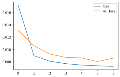
losses = pd.DataFrame(model.history.history)
losses.plot()
<AxesSubplot:>
Evaluate on Test Data
first_eval_batch = scaled_train[-length:]
first_eval_batch
array([[0.1038961 , 0.        , 0.72231687, ..., 0.53550296, 0.15909546,
        0.15909546],
       [0.11688312, 0.        , 0.73424191, ..., 0.52662722, 0.40344207,
        0.40344207],
       [0.11688312, 0.        , 0.73424191, ..., 0.51775148, 0.20452271,
        0.20452271],
       ...,
       [0.18181818, 0.        , 0.70017036, ..., 0.50118343, 0.33340004,
        0.33340004],
       [0.09090909, 0.        , 0.70017036, ..., 0.51952663, 0.78747248,
        0.78747248],
       [0.1038961 , 0.        , 0.70017036, ..., 0.53846154, 0.77286372,
        0.77286372]])
first_eval_batch = first_eval_batch.reshape((1, length, scaled_train.shape[1]))
model.predict(first_eval_batch)
array([[ 0.12962861,  0.11173069,  0.7100676 ,  0.39257962,  0.5337119 ,
         0.4407935 ,  0.43118235,  0.4344098 ,  0.7135023 ,  0.3761254 ,
         0.328368  ,  0.37035555,  0.6467758 , -0.00678065,  0.62732697,
         0.40806448,  0.50039965,  0.33460236,  0.5257516 ,  0.35319155,
         0.6283157 ,  0.5327904 ,  0.43472147,  0.19735846,  0.6059718 ,
         0.5548344 ,  0.5132371 ,  0.5090848 ]], dtype=float32)
scaled_test[0]
array([0.19480519, 0.        , 0.70017036, 0.3920434 , 0.53007217,
       0.41064526, 0.40616246, 0.41913319, 0.72714286, 0.4115245 ,
       0.30722892, 0.36445121, 0.66777778, 0.        , 0.61119082,
       0.39840637, 0.51618399, 0.32953105, 0.53703704, 0.34024896,
       0.6057377 , 0.52631579, 0.41881579, 0.2       , 0.55283333,
       0.53372781, 0.76305783, 0.76305783])
n_features = scaled_train.shape[1]
test_predictions = []

first_eval_batch = scaled_train[-length:]
current_batch = first_eval_batch.reshape((1, length, n_features))

for i in range(len(test)):
    current_pred = model.predict(current_batch)[0]
    test_predictions.append(current_pred)
    current_batch = np.append(current_batch[:, 1:, :],[[current_pred]], axis=1)
scaled_test
array([[0.19480519, 0.        , 0.70017036, ..., 0.53372781, 0.76305783,
        0.76305783],
       [0.37662338, 0.        , 0.70017036, ..., 0.52840237, 0.62337402,
        0.62337402],
       [0.12987013, 0.        , 0.70017036, ..., 0.52366864, 0.08785271,
        0.08785271],
       ...,
       [0.32467532, 0.33333333, 0.87052811, ..., 0.86804734, 0.58415049,
        0.58415049],
       [0.51948052, 0.33333333, 0.87052811, ..., 0.86568047, 0.12627577,
        0.12627577],
       [0.53246753, 0.33333333, 0.87052811, ..., 0.86390533, 0.68260957,
        0.68260957]])
Inverse Transformations and Compare
true_predictions = scaler.inverse_transform(test_predictions)
true_predictions
array([[119.81403247,   3.35192084,  24.55809664, ...,   7.97670179,
         25.65645882,  25.44896849],
       [135.39294168,   5.15252039,  24.49285675, ...,   8.37637454,
         25.66081033,  25.26328633],
       [144.21259135,   6.69974104,  24.44082725, ...,   8.80649047,
         25.73894385,  25.18596294],
       ...,
       [222.21735567,  16.03211939,  24.13516293, ...,  21.59099305,
         23.42215515,  22.95250515],
       [222.21735567,  16.03211939,  24.13516363, ...,  21.59099506,
         23.42215218,  22.95250515],
       [222.21733272,  16.03211939,  24.13516398, ...,  21.59099103,
         23.42215218,  22.95250217]])
pred_df = pd.DataFrame(data=true_predictions, index=test.index, columns = test.columns)
test
| Appliances | lights | T1 | RH_1 | T2 | RH_2 | T3 | RH_3 | T4 | RH_4 | ... | T9 | RH_9 | T_out | Press_mm_hg | RH_out | Windspeed | Visibility | Tdewpoint | rv1 | rv2 | |
|---|---|---|---|---|---|---|---|---|---|---|---|---|---|---|---|---|---|---|---|---|---|
| date | |||||||||||||||||||||
| 2016-05-25 18:10:00 | 170 | 0 | 24.50 | 37.86 | 24.00 | 34.27 | 25.00 | 36.70 | 24.29 | 37.79 | ... | 22.00 | 37.23 | 16.48 | 756.1 | 55.83 | 2.00 | 38.17 | 7.62 | 38.14 | 38.14 |
| 2016-05-25 18:20:00 | 310 | 0 | 24.50 | 37.30 | 23.86 | 34.33 | 24.94 | 36.67 | 24.29 | 37.79 | ... | 22.00 | 37.36 | 16.47 | 756.1 | 55.67 | 2.00 | 36.33 | 7.53 | 31.16 | 31.16 |
| 2016-05-25 18:30:00 | 120 | 0 | 24.50 | 36.96 | 23.73 | 34.33 | 24.85 | 36.50 | 24.29 | 37.79 | ... | 22.03 | 37.39 | 16.45 | 756.1 | 55.50 | 2.00 | 34.50 | 7.45 | 4.40 | 4.40 |
| 2016-05-25 18:40:00 | 120 | 0 | 24.50 | 37.00 | 23.70 | 34.40 | 24.84 | 36.45 | 24.29 | 37.90 | ... | 22.10 | 37.72 | 16.43 | 756.1 | 55.33 | 2.00 | 32.67 | 7.37 | 27.12 | 27.12 |
| 2016-05-25 18:50:00 | 120 | 0 | 24.49 | 37.07 | 23.68 | 34.52 | 24.84 | 36.49 | 24.28 | 37.93 | ... | 22.10 | 37.81 | 16.42 | 756.1 | 55.17 | 2.00 | 30.83 | 7.28 | 10.27 | 10.27 |
| ... | ... | ... | ... | ... | ... | ... | ... | ... | ... | ... | ... | ... | ... | ... | ... | ... | ... | ... | ... | ... | ... |
| 2016-05-27 17:20:00 | 100 | 0 | 25.57 | 46.56 | 25.89 | 42.03 | 27.20 | 41.16 | 24.70 | 45.59 | ... | 23.20 | 46.79 | 22.73 | 755.2 | 55.67 | 3.33 | 23.67 | 13.33 | 43.10 | 43.10 |
| 2016-05-27 17:30:00 | 90 | 0 | 25.50 | 46.50 | 25.75 | 42.08 | 27.13 | 41.22 | 24.70 | 45.59 | ... | 23.20 | 46.79 | 22.60 | 755.2 | 56.00 | 3.50 | 24.50 | 13.30 | 49.28 | 49.28 |
| 2016-05-27 17:40:00 | 270 | 10 | 25.50 | 46.60 | 25.63 | 42.77 | 27.05 | 41.69 | 24.70 | 45.73 | ... | 23.20 | 46.79 | 22.47 | 755.2 | 56.33 | 3.67 | 25.33 | 13.27 | 29.20 | 29.20 |
| 2016-05-27 17:50:00 | 420 | 10 | 25.50 | 46.99 | 25.41 | 43.04 | 26.89 | 41.29 | 24.70 | 45.79 | ... | 23.20 | 46.82 | 22.33 | 755.2 | 56.67 | 3.83 | 26.17 | 13.23 | 6.32 | 6.32 |
| 2016-05-27 18:00:00 | 430 | 10 | 25.50 | 46.60 | 25.26 | 42.97 | 26.82 | 41.16 | 24.70 | 45.96 | ... | 23.20 | 46.84 | 22.20 | 755.2 | 57.00 | 4.00 | 27.00 | 13.20 | 34.12 | 34.12 |
288 rows × 28 columns
pred_df
| Appliances | lights | T1 | RH_1 | T2 | RH_2 | T3 | RH_3 | T4 | RH_4 | ... | T9 | RH_9 | T_out | Press_mm_hg | RH_out | Windspeed | Visibility | Tdewpoint | rv1 | rv2 | |
|---|---|---|---|---|---|---|---|---|---|---|---|---|---|---|---|---|---|---|---|---|---|
| date | |||||||||||||||||||||
| 2016-05-25 18:10:00 | 119.814032 | 3.351921 | 24.558097 | 37.874826 | 24.045388 | 35.283886 | 25.178642 | 36.989033 | 24.194516 | 37.009804 | ... | 21.939059 | 37.510725 | 17.030903 | 756.247622 | 57.038832 | 1.973585 | 41.358309 | 7.976702 | 25.656459 | 25.448968 |
| 2016-05-25 18:20:00 | 135.392942 | 5.152520 | 24.492857 | 37.657199 | 23.754765 | 35.277770 | 25.187547 | 37.040140 | 24.122789 | 36.663892 | ... | 21.886550 | 37.796598 | 17.147620 | 756.141145 | 57.685050 | 1.954602 | 41.986854 | 8.376375 | 25.660810 | 25.263286 |
| 2016-05-25 18:30:00 | 144.212591 | 6.699741 | 24.440827 | 37.524560 | 23.471283 | 35.436711 | 25.215640 | 37.063246 | 24.070092 | 36.440047 | ... | 21.844848 | 38.057945 | 17.257024 | 755.974725 | 58.609539 | 1.932213 | 42.552782 | 8.806490 | 25.738944 | 25.185963 |
| 2016-05-25 18:40:00 | 149.768802 | 8.069998 | 24.386769 | 37.446713 | 23.180236 | 35.667879 | 25.250065 | 37.088631 | 24.017115 | 36.277079 | ... | 21.810150 | 38.261318 | 17.332690 | 755.705818 | 59.766602 | 1.899848 | 42.988523 | 9.248289 | 25.786471 | 25.105795 |
| 2016-05-25 18:50:00 | 153.218038 | 9.331562 | 24.329630 | 37.435610 | 22.893000 | 35.979222 | 25.289133 | 37.152087 | 23.964464 | 36.188050 | ... | 21.782987 | 38.419516 | 17.376678 | 755.337311 | 61.196783 | 1.864786 | 43.348687 | 9.716914 | 25.818307 | 25.025800 |
| ... | ... | ... | ... | ... | ... | ... | ... | ... | ... | ... | ... | ... | ... | ... | ... | ... | ... | ... | ... | ... | ... |
| 2016-05-27 17:20:00 | 222.217310 | 16.032119 | 24.135162 | 60.898420 | 22.814009 | 60.913240 | 27.341344 | 52.462853 | 25.639273 | 52.654667 | ... | 27.455314 | 61.039082 | 22.957183 | 722.226312 | 84.129677 | 3.372346 | 56.142634 | 21.590995 | 23.422155 | 22.952505 |
| 2016-05-27 17:30:00 | 222.217333 | 16.032119 | 24.135162 | 60.898420 | 22.814009 | 60.913240 | 27.341345 | 52.462853 | 25.639273 | 52.654667 | ... | 27.455314 | 61.039084 | 22.957180 | 722.226312 | 84.129681 | 3.372346 | 56.142634 | 21.590993 | 23.422155 | 22.952502 |
| 2016-05-27 17:40:00 | 222.217356 | 16.032119 | 24.135163 | 60.898420 | 22.814007 | 60.913240 | 27.341345 | 52.462853 | 25.639273 | 52.654667 | ... | 27.455313 | 61.039084 | 22.957180 | 722.226312 | 84.129677 | 3.372346 | 56.142631 | 21.590993 | 23.422155 | 22.952505 |
| 2016-05-27 17:50:00 | 222.217356 | 16.032119 | 24.135164 | 60.898420 | 22.814009 | 60.913240 | 27.341347 | 52.462853 | 25.639273 | 52.654667 | ... | 27.455313 | 61.039087 | 22.957183 | 722.226312 | 84.129672 | 3.372346 | 56.142631 | 21.590995 | 23.422152 | 22.952505 |
| 2016-05-27 18:00:00 | 222.217333 | 16.032119 | 24.135164 | 60.898420 | 22.814011 | 60.913240 | 27.341347 | 52.462853 | 25.639273 | 52.654667 | ... | 27.455313 | 61.039092 | 22.957183 | 722.226309 | 84.129672 | 3.372347 | 56.142631 | 21.590991 | 23.422152 | 22.952502 |
288 rows × 28 columns
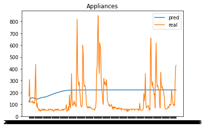
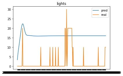
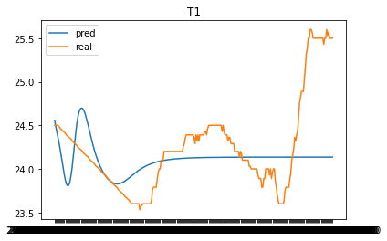
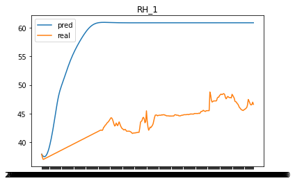
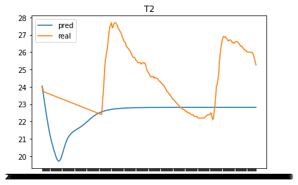
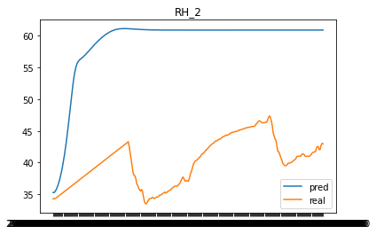
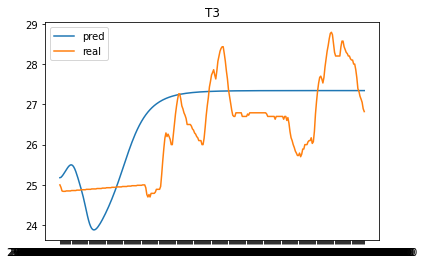
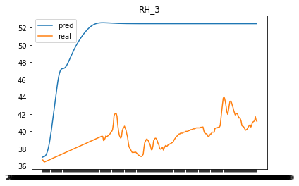
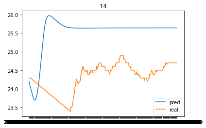
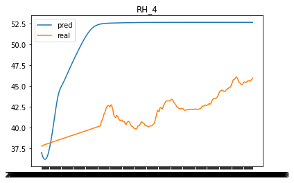
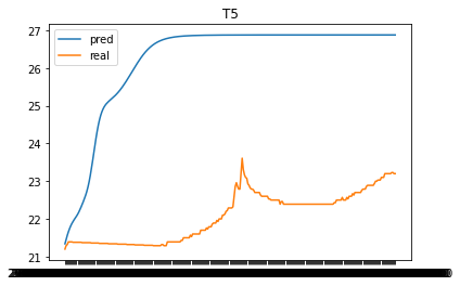
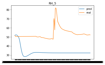
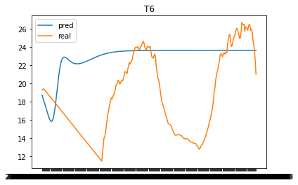
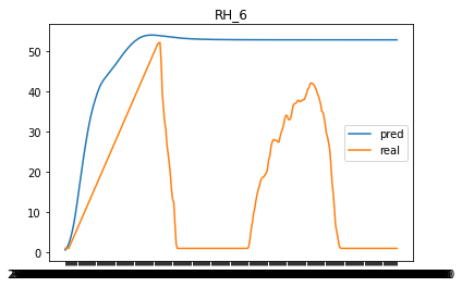
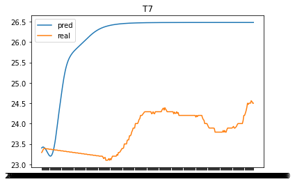
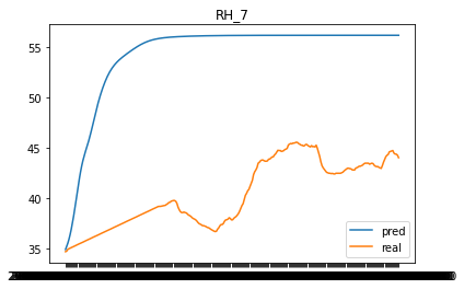
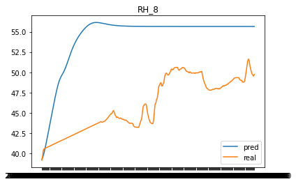
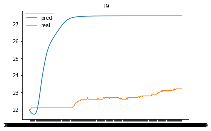
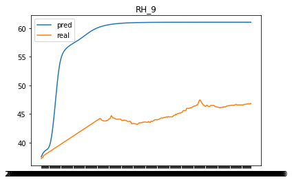
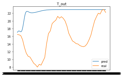
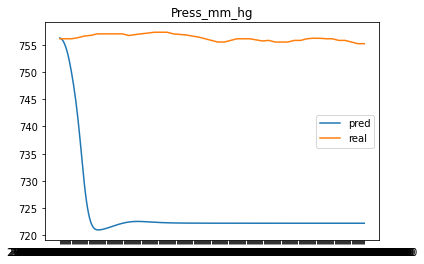
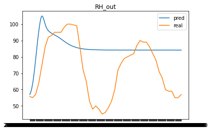
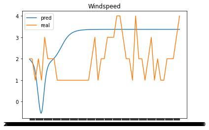
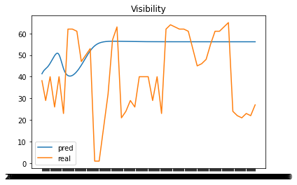
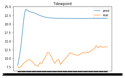
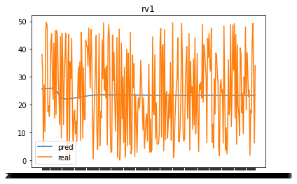
columns = pred_df.columns
for col in columns:
    plt.plot(pred_df[col], label='pred')
    plt.plot(test[col], label='real')
    plt.legend()
    plt.title(col)
    plt.show()