Time Series Analysis - VAR Models
VAR Model
import numpy as np
import pandas as pd
%matplotlib inline

from statsmodels.tsa.api import VAR
from statsmodels.tsa.stattools import adfuller
from statsmodels.tools.eval_measures import rmse

import warnings
warnings.filterwarnings('ignore')

df = pd.read_csv('Data/M2SLMoneyStock.csv', index_col=0, parse_dates=True)
df.index.freq = 'MS'

sp = pd.read_csv('Data/PCEPersonalSpending.csv', index_col=0, parse_dates=True)
sp.index.freq = 'MS'
df.head()
| Money | |
|---|---|
| Date | |
| 1995-01-01 | 3492.4 |
| 1995-02-01 | 3489.9 |
| 1995-03-01 | 3491.1 |
| 1995-04-01 | 3499.2 |
| 1995-05-01 | 3524.2 |
sp.head()
| Spending | |
|---|---|
| Date | |
| 1995-01-01 | 4851.2 |
| 1995-02-01 | 4850.8 |
| 1995-03-01 | 4885.4 |
| 1995-04-01 | 4890.2 |
| 1995-05-01 | 4933.1 |
df = df.join(sp)
df.head()
| Money | Spending | |
|---|---|---|
| Date | ||
| 1995-01-01 | 3492.4 | 4851.2 |
| 1995-02-01 | 3489.9 | 4850.8 |
| 1995-03-01 | 3491.1 | 4885.4 |
| 1995-04-01 | 3499.2 | 4890.2 |
| 1995-05-01 | 3524.2 | 4933.1 |
df.shape
(252, 2)
df = df.dropna()
df.shape
(252, 2)
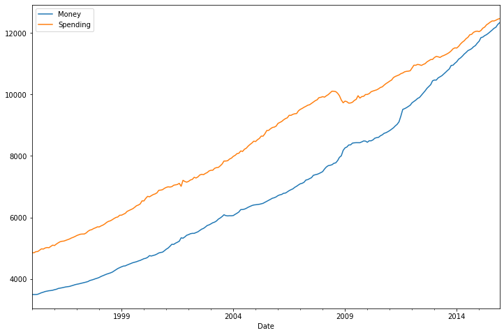
df.plot(figsize=(12,8))
<AxesSubplot:xlabel='Date'>
Differencing
def adf_test(series, title=''):
    """
    Pass in a time series and an optional title, returns an ADF report
    """
    print(f'Augmented Dickey-Fuller Test: {title}')
    result = adfuller(series.dropna(), autolag = 'AIC')

    labels = ['ADF test statistic', 'p-value', '# lags used', '# obervations']
    out = pd.Series(result[0:4], index = labels)

    for key, val in result[4].items():
        out[f'critical value ({key})'] = val

    print(out.to_string())

    if result[1] <= 0.05:
        print('Strong evidence against the null hypothesis')
        print('Reject the null hypothesis')
        print('Data has no unit root and is stationary')
    else:
        print('Weak evidence against the null hypothesis')
        print('Fail to reject the null hypothesis')
        print('Data has a unit root and is non-stationary')
adf_test(df['Money'])
Augmented Dickey-Fuller Test:
ADF test statistic        4.239022
p-value                   1.000000
# lags used               4.000000
# obervations           247.000000
critical value (1%)      -3.457105
critical value (5%)      -2.873314
critical value (10%)     -2.573044
Weak evidence against the null hypothesis
Fail to reject the null hypothesis
Data has a unit root and is non-stationary
adf_test(df['Spending'])
Augmented Dickey-Fuller Test:
ADF test statistic        0.149796
p-value                   0.969301
# lags used               3.000000
# obervations           248.000000
critical value (1%)      -3.456996
critical value (5%)      -2.873266
critical value (10%)     -2.573019
Weak evidence against the null hypothesis
Fail to reject the null hypothesis
Data has a unit root and is non-stationary
df_transformed = df.diff()
print(adf_test(df_transformed['Money']))
print(adf_test(df_transformed['Spending']))
Augmented Dickey-Fuller Test:
ADF test statistic       -2.057404
p-value                   0.261984
# lags used              15.000000
# obervations           235.000000
critical value (1%)      -3.458487
critical value (5%)      -2.873919
critical value (10%)     -2.573367
Weak evidence against the null hypothesis
Fail to reject the null hypothesis
Data has a unit root and is non-stationary
None
Augmented Dickey-Fuller Test:
ADF test statistic     -7.226974e+00
p-value                 2.041027e-10
# lags used             2.000000e+00
# obervations           2.480000e+02
critical value (1%)    -3.456996e+00
critical value (5%)    -2.873266e+00
critical value (10%)   -2.573019e+00
Strong evidence against the null hypothesis
Reject the null hypothesis
Data has no unit root and is stationary
None
df_transformed = df_transformed.diff().dropna()
df_transformed
| Money | Spending | |
|---|---|---|
| Date | ||
| 1995-03-01 | 3.7 | 35.0 |
| 1995-04-01 | 6.9 | -29.8 |
| 1995-05-01 | 16.9 | 38.1 |
| 1995-06-01 | -0.3 | 1.5 |
| 1995-07-01 | -6.2 | -51.7 |
| ... | ... | ... |
| 2015-08-01 | -0.7 | -8.5 |
| 2015-09-01 | 5.5 | -39.8 |
| 2015-10-01 | -23.1 | 24.5 |
| 2015-11-01 | 55.8 | 10.7 |
| 2015-12-01 | -31.2 | -15.0 |
250 rows × 2 columns
print(adf_test(df_transformed['Money']))
print(adf_test(df_transformed['Spending']))
Augmented Dickey-Fuller Test:
ADF test statistic     -7.077471e+00
p-value                 4.760675e-10
# lags used             1.400000e+01
# obervations           2.350000e+02
critical value (1%)    -3.458487e+00
critical value (5%)    -2.873919e+00
critical value (10%)   -2.573367e+00
Strong evidence against the null hypothesis
Reject the null hypothesis
Data has no unit root and is stationary
None
Augmented Dickey-Fuller Test:
ADF test statistic     -8.760145e+00
p-value                 2.687900e-14
# lags used             8.000000e+00
# obervations           2.410000e+02
critical value (1%)    -3.457779e+00
critical value (5%)    -2.873609e+00
critical value (10%)   -2.573202e+00
Strong evidence against the null hypothesis
Reject the null hypothesis
Data has no unit root and is stationary
None
Train and Test Split
# Number of Obervations
nobs = 12
train = df_transformed[:-nobs]
test = df_transformed[-nobs:]
print(train.shape)
print(test.shape)
(238, 2)
(12, 2)
GRIDSEARCH FOR ORDER p AR of VAR model
model = VAR(train)

for p in [1,2,3,4,5,6,7]:
    results = model.fit(p)
    print(f'ORDER {p}')
    print(f'AIC: {results.aic}')
    print('\n')
ORDER 1
AIC: 14.178610495220896


ORDER 2
AIC: 13.955189367163703


ORDER 3
AIC: 13.849518291541038


ORDER 4
AIC: 13.827950574458283


ORDER 5
AIC: 13.78730034460964


ORDER 6
AIC: 13.799076756885809


ORDER 7
AIC: 13.797638727913972
results = model.fit(5)
results.summary()
  Summary of Regression Results
==================================
Model:                         VAR
Method:                        OLS
Date:           Fri, 16, Oct, 2020
Time:                     12:55:32
--------------------------------------------------------------------
No. of Equations:         2.00000    BIC:                    14.1131
Nobs:                     233.000    HQIC:                   13.9187
Log likelihood:          -2245.45    FPE:                    972321.
AIC:                      13.7873    Det(Omega_mle):         886628.
--------------------------------------------------------------------
Results for equation Money
==============================================================================
                 coefficient       std. error           t-stat            prob
------------------------------------------------------------------------------
const               0.516683         1.782238            0.290           0.772
L1.Money           -0.646232         0.068177           -9.479           0.000
L1.Spending        -0.107411         0.051388           -2.090           0.037
L2.Money           -0.497482         0.077749           -6.399           0.000
L2.Spending        -0.192202         0.068613           -2.801           0.005
L3.Money           -0.234442         0.081004           -2.894           0.004
L3.Spending        -0.178099         0.074288           -2.397           0.017
L4.Money           -0.295531         0.075294           -3.925           0.000
L4.Spending        -0.035564         0.069664           -0.511           0.610
L5.Money           -0.162399         0.066700           -2.435           0.015
L5.Spending        -0.058449         0.051357           -1.138           0.255
==============================================================================

Results for equation Spending
==============================================================================
                 coefficient       std. error           t-stat            prob
------------------------------------------------------------------------------
const               0.203469         2.355446            0.086           0.931
L1.Money            0.188105         0.090104            2.088           0.037
L1.Spending        -0.878970         0.067916          -12.942           0.000
L2.Money            0.053017         0.102755            0.516           0.606
L2.Spending        -0.625313         0.090681           -6.896           0.000
L3.Money           -0.022172         0.107057           -0.207           0.836
L3.Spending        -0.389041         0.098180           -3.963           0.000
L4.Money           -0.170456         0.099510           -1.713           0.087
L4.Spending        -0.245435         0.092069           -2.666           0.008
L5.Money           -0.083165         0.088153           -0.943           0.345
L5.Spending        -0.181699         0.067874           -2.677           0.007
==============================================================================

Correlation matrix of residuals
               Money  Spending
Money       1.000000 -0.267934
Spending   -0.267934  1.000000
# Grab 5 Lagged values, right before the test starts!
# Numpy array
lagged_values = train.values[-5:]
z = results.forecast(y=lagged_values, steps = 12)
z
array([[-16.99527634,  36.14982003],
       [ -3.17403756, -11.45029844],
       [ -0.377725  ,  -6.68496939],
       [ -2.60223305,   5.47945777],
       [  4.228557  ,  -2.44336505],
       [  1.55939341,   0.38763902],
       [ -0.99841027,   3.88368011],
       [  0.36451042,  -2.3561014 ],
       [ -1.21062726,  -1.22414652],
       [  0.22587712,   0.786927  ],
       [  1.33893884,   0.18097449],
       [ -0.21858453,   0.21275046]])
test
| Money | Spending | |
|---|---|---|
| Date | ||
| 2015-01-01 | -15.5 | -26.6 |
| 2015-02-01 | 56.1 | 52.4 |
| 2015-03-01 | -102.8 | 39.5 |
| 2015-04-01 | 30.9 | -40.4 |
| 2015-05-01 | -15.8 | 38.8 |
| 2015-06-01 | 14.0 | -34.1 |
| 2015-07-01 | 6.7 | 6.9 |
| 2015-08-01 | -0.7 | -8.5 |
| 2015-09-01 | 5.5 | -39.8 |
| 2015-10-01 | -23.1 | 24.5 |
| 2015-11-01 | 55.8 | 10.7 |
| 2015-12-01 | -31.2 | -15.0 |
idx = pd.date_range('2015-01-01', periods=12, freq = 'MS')
idx
DatetimeIndex(['2015-01-01', '2015-02-01', '2015-03-01', '2015-04-01',
               '2015-05-01', '2015-06-01', '2015-07-01', '2015-08-01',
               '2015-09-01', '2015-10-01', '2015-11-01', '2015-12-01'],
              dtype='datetime64[ns]', freq='MS')
df_forecast = pd.DataFrame(data=z, index=idx, columns=['Money_2d', 'Spending_2d'])
df_forecast
| Money_2d | Spending_2d | |
|---|---|---|
| 2015-01-01 | -16.995276 | 36.149820 |
| 2015-02-01 | -3.174038 | -11.450298 |
| 2015-03-01 | -0.377725 | -6.684969 |
| 2015-04-01 | -2.602233 | 5.479458 |
| 2015-05-01 | 4.228557 | -2.443365 |
| 2015-06-01 | 1.559393 | 0.387639 |
| 2015-07-01 | -0.998410 | 3.883680 |
| 2015-08-01 | 0.364510 | -2.356101 |
| 2015-09-01 | -1.210627 | -1.224147 |
| 2015-10-01 | 0.225877 | 0.786927 |
| 2015-11-01 | 1.338939 | 0.180974 |
| 2015-12-01 | -0.218585 | 0.212750 |
Invert the Transformation
df_forecast['Money_1d'] = (df['Money'].iloc[-nobs-1]-df['Money'].iloc[-nobs-2]) + df_forecast['Money_2d'].cumsum()

df_forecast['MoneyForecast'] = df['Money'].iloc[-nobs-1] + df_forecast['Money_1d'].cumsum()
df_forecast['Spending_1d'] = (df['Spending'].iloc[-nobs-1]-df['Spending'].iloc[-nobs-2]) + df_forecast['Spending_2d'].cumsum()

df_forecast['SpendingForecast'] = df['Spending'].iloc[-nobs-1] + df_forecast['Spending_1d'].cumsum()
df_forecast.head()
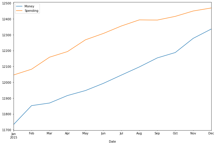
test_range = df[-nobs:]
test_range.plot(figsize = (12,8))
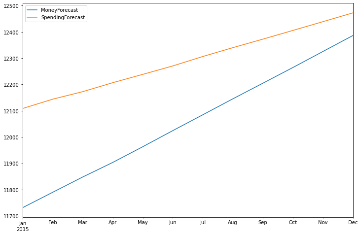
df_forecast[['MoneyForecast','SpendingForecast']].plot(figsize=(12,8))
<AxesSubplot:>
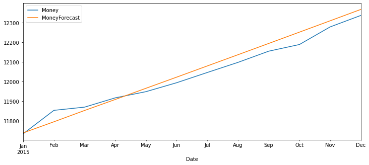
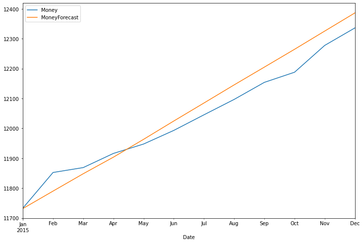
test_range['Money'].plot(legend=True, figsize=(12,8))
df_forecast['MoneyForecast'].plot(legend=True)
<AxesSubplot:xlabel='Date'>
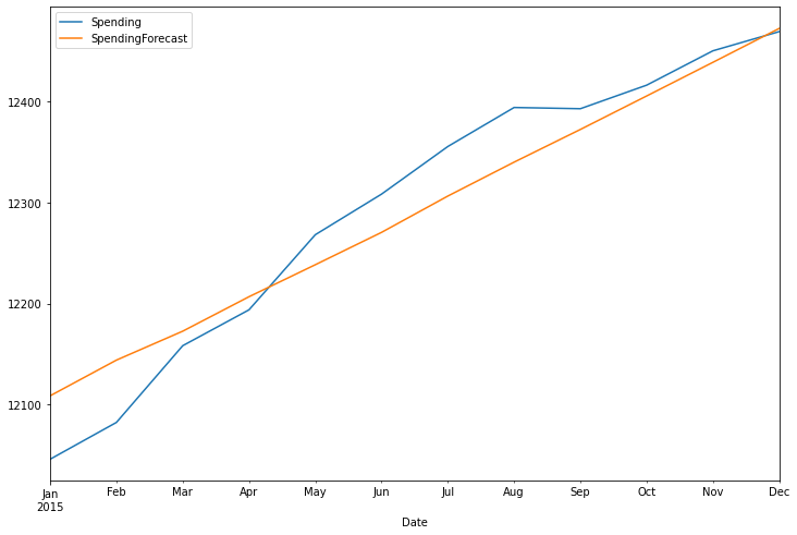
test_range['Spending'].plot(legend=True, figsize=(12,8))
df_forecast['SpendingForecast'].plot(legend=True)
<AxesSubplot:xlabel='Date'>
rmse(test_range['Money'], df_forecast['MoneyForecast'])
43.71049653558893
test_range['Money'].mean()
12034.008333333333
rmse(test_range['Spending'], df_forecast['SpendingForecast'])
37.001175169408036
test_range['Spending'].mean()
12294.533333333335
VARMA Model
import numpy as np
import pandas as pd
%matplotlib inline

from statsmodels.tsa.statespace.varmax import VARMAX, VARMAXResults
from statsmodels.tsa.stattools import adfuller
from pmdarima import auto_arima
from statsmodels.tools.eval_measures import rmse

import warnings
warnings.filterwarnings('ignore')

df = pd.read_csv('Data/M2SLMoneyStock.csv', index_col=0, parse_dates=True)
df.index.freq = 'MS'

sp = pd.read_csv('Data/PCEPersonalSpending.csv', index_col=0, parse_dates=True)
sp.index.freq = 'MS'
df = df.join(sp)
df
| Money | Spending | |
|---|---|---|
| Date | ||
| 1995-01-01 | 3492.4 | 4851.2 |
| 1995-02-01 | 3489.9 | 4850.8 |
| 1995-03-01 | 3491.1 | 4885.4 |
| 1995-04-01 | 3499.2 | 4890.2 |
| 1995-05-01 | 3524.2 | 4933.1 |
| ... | ... | ... |
| 2015-08-01 | 12096.8 | 12394.0 |
| 2015-09-01 | 12153.8 | 12392.8 |
| 2015-10-01 | 12187.7 | 12416.1 |
| 2015-11-01 | 12277.4 | 12450.1 |
| 2015-12-01 | 12335.9 | 12469.1 |
252 rows × 2 columns
auto_arima(df['Money'], maxiter=1000)
ARIMA(maxiter=1000, order=(1, 2, 1), scoring_args={}, with_intercept=False)
auto_arima(df['Spending'], maxiter = 1000)
ARIMA(maxiter=1000, order=(1, 1, 2), scoring_args={})
df_transformed = df.diff().diff()
df_transformed = df_transformed.dropna()
df_transformed.head()
| Money | Spending | |
|---|---|---|
| Date | ||
| 1995-03-01 | 3.7 | 35.0 |
| 1995-04-01 | 6.9 | -29.8 |
| 1995-05-01 | 16.9 | 38.1 |
| 1995-06-01 | -0.3 | 1.5 |
| 1995-07-01 | -6.2 | -51.7 |
len(df_transformed)
250
Train / Test Split
nobs = 12
train, test = df_transformed[0:-nobs], df_transformed[-nobs:]
print(train.shape)
print(test.shape)
(238, 2)
(12, 2)
Fit the VARMA(1,2) Model
model = VARMAX(train, order=(1,2), trend='c')
results = model.fit(maxiter = 1000, disp=False)
results.summary()
| Dep. Variable: | ['Money', 'Spending'] | No. Observations: | 238 |
|---|---|---|---|
| Model: | VARMA(1,2) | Log Likelihood | -2285.860 |
| + intercept | AIC | 4605.720 | |
| Date: | Fri, 16 Oct 2020 | BIC | 4664.749 |
| Time: | 13:32:48 | HQIC | 4629.510 |
| Sample: | 03-01-1995 | ||
| - 12-01-2014 | |||
| Covariance Type: | opg |
| Ljung-Box (Q): | 67.60, 28.85 | Jarque-Bera (JB): | 552.05, 127.75 |
|---|---|---|---|
| Prob(Q): | 0.00, 0.90 | Prob(JB): | 0.00, 0.00 |
| Heteroskedasticity (H): | 5.55, 2.87 | Skew: | 1.34, -0.32 |
| Prob(H) (two-sided): | 0.00, 0.00 | Kurtosis: | 9.96, 6.53 |
| coef | std err | z | P>|z| | [0.025 | 0.975] | |
|---|---|---|---|---|---|---|
| intercept | 0.1643 | 0.861 | 0.191 | 0.849 | -1.523 | 1.852 |
| L1.Money | -1.1746 | 4.475 | -0.262 | 0.793 | -9.945 | 7.596 |
| L1.Spending | 2.5441 | 8.612 | 0.295 | 0.768 | -14.335 | 19.423 |
| L1.e(Money) | 0.4093 | 4.462 | 0.092 | 0.927 | -8.337 | 9.155 |
| L1.e(Spending) | -2.6706 | 8.613 | -0.310 | 0.757 | -19.553 | 14.212 |
| L2.e(Money) | -1.4619 | 4.634 | -0.315 | 0.752 | -10.544 | 7.620 |
| L2.e(Spending) | 2.3604 | 7.599 | 0.311 | 0.756 | -12.534 | 17.254 |
| coef | std err | z | P>|z| | [0.025 | 0.975] | |
|---|---|---|---|---|---|---|
| intercept | 0.0757 | 0.070 | 1.079 | 0.281 | -0.062 | 0.213 |
| L1.Money | -0.3230 | 2.423 | -0.133 | 0.894 | -5.072 | 4.426 |
| L1.Spending | 0.8097 | 4.508 | 0.180 | 0.857 | -8.027 | 9.646 |
| L1.e(Money) | 0.4454 | 2.485 | 0.179 | 0.858 | -4.425 | 5.316 |
| L1.e(Spending) | -1.7643 | 4.485 | -0.393 | 0.694 | -10.556 | 7.027 |
| L2.e(Money) | -0.4424 | 2.579 | -0.172 | 0.864 | -5.497 | 4.613 |
| L2.e(Spending) | 0.7857 | 3.941 | 0.199 | 0.842 | -6.939 | 8.511 |
| coef | std err | z | P>|z| | [0.025 | 0.975] | |
|---|---|---|---|---|---|---|
| sqrt.var.Money | 25.7081 | 1.888 | 13.619 | 0.000 | 22.008 | 29.408 |
| sqrt.cov.Money.Spending | -8.7303 | 1.843 | -4.738 | 0.000 | -12.342 | -5.119 |
| sqrt.var.Spending | 33.4869 | 1.234 | 27.128 | 0.000 | 31.068 | 35.906 |
Warnings:
[1] Covariance matrix calculated using the outer product of gradients (complex-step).
Predict the next 12 values
df_forecast = results.forecast(12)
df_forecast
| Money | Spending | |
|---|---|---|
| 2015-01-01 | -11.050219 | 37.367991 |
| 2015-02-01 | -11.097937 | -4.699904 |
| 2015-03-01 | 1.242635 | -0.144623 |
| 2015-04-01 | -1.663244 | -0.442775 |
| 2015-05-01 | 0.991430 | 0.254518 |
| 2015-06-01 | -0.352719 | -0.038456 |
| 2015-07-01 | 0.480741 | 0.158538 |
| 2015-08-01 | 0.002947 | 0.048803 |
| 2015-09-01 | 0.284976 | 0.114297 |
| 2015-10-01 | 0.120333 | 0.076220 |
| 2015-11-01 | 0.216849 | 0.098576 |
| 2015-12-01 | 0.160359 | 0.085499 |
Invert the Transformation
df_forecast['Money_1d'] = (df['Money'].iloc[-nobs-1]-df['Money'].iloc[-nobs-2]) + df_forecast['Money'].cumsum()

df_forecast['MoneyForecast'] = df['Money'].iloc[-nobs-1] + df_forecast['Money_1d'].cumsum()
df_forecast['Spending_1d'] = (df['Spending'].iloc[-nobs-1]-df['Spending'].iloc[-nobs-2]) + df_forecast['Spending'].cumsum()

df_forecast['SpendingForecast'] = df['Spending'].iloc[-nobs-1] + df_forecast['Spending_1d'].cumsum()
df_forecast
| Money | Spending | Money_1d | MoneyForecast | Spending_1d | SpendingForecast | |
|---|---|---|---|---|---|---|
| 2015-01-01 | -11.050219 | 37.367991 | 67.549781 | 11737.649781 | 47.967991 | 12109.967991 |
| 2015-02-01 | -11.097937 | -4.699904 | 56.451845 | 11794.101626 | 43.268087 | 12153.236078 |
| 2015-03-01 | 1.242635 | -0.144623 | 57.694479 | 11851.796105 | 43.123464 | 12196.359542 |
| 2015-04-01 | -1.663244 | -0.442775 | 56.031235 | 11907.827340 | 42.680689 | 12239.040232 |
| 2015-05-01 | 0.991430 | 0.254518 | 57.022665 | 11964.850005 | 42.935207 | 12281.975439 |
| 2015-06-01 | -0.352719 | -0.038456 | 56.669946 | 12021.519951 | 42.896751 | 12324.872190 |
| 2015-07-01 | 0.480741 | 0.158538 | 57.150687 | 12078.670637 | 43.055290 | 12367.927480 |
| 2015-08-01 | 0.002947 | 0.048803 | 57.153633 | 12135.824271 | 43.104092 | 12411.031572 |
| 2015-09-01 | 0.284976 | 0.114297 | 57.438610 | 12193.262881 | 43.218389 | 12454.249961 |
| 2015-10-01 | 0.120333 | 0.076220 | 57.558942 | 12250.821823 | 43.294609 | 12497.544570 |
| 2015-11-01 | 0.216849 | 0.098576 | 57.775792 | 12308.597615 | 43.393185 | 12540.937754 |
| 2015-12-01 | 0.160359 | 0.085499 | 57.936150 | 12366.533765 | 43.478684 | 12584.416438 |
pd.concat([df.iloc[-12:], df_forecast[['MoneyForecast','SpendingForecast']]], axis=1)
| Money | Spending | MoneyForecast | SpendingForecast | |
|---|---|---|---|---|
| Date | ||||
| 2015-01-01 | 11733.2 | 12046.0 | 11737.649781 | 12109.967991 |
| 2015-02-01 | 11852.4 | 12082.4 | 11794.101626 | 12153.236078 |
| 2015-03-01 | 11868.8 | 12158.3 | 11851.796105 | 12196.359542 |
| 2015-04-01 | 11916.1 | 12193.8 | 11907.827340 | 12239.040232 |
| 2015-05-01 | 11947.6 | 12268.1 | 11964.850005 | 12281.975439 |
| 2015-06-01 | 11993.1 | 12308.3 | 12021.519951 | 12324.872190 |
| 2015-07-01 | 12045.3 | 12355.4 | 12078.670637 | 12367.927480 |
| 2015-08-01 | 12096.8 | 12394.0 | 12135.824271 | 12411.031572 |
| 2015-09-01 | 12153.8 | 12392.8 | 12193.262881 | 12454.249961 |
| 2015-10-01 | 12187.7 | 12416.1 | 12250.821823 | 12497.544570 |
| 2015-11-01 | 12277.4 | 12450.1 | 12308.597615 | 12540.937754 |
| 2015-12-01 | 12335.9 | 12469.1 | 12366.533765 | 12584.416438 |
Plots
df['Money'][-nobs:].plot(figsize=(12,5), legend=True).autoscale(axis='x', tight=True)
df_forecast['MoneyForecast'].plot(legend=True)
<AxesSubplot:xlabel='Date'>