Deep Learning from Scratch - Back Propagation (1)
Computational Graph
여러개의 Node와 Edge로 표현된다. 계산과정을 그래프로 나타낸것.
국소적 계산
계산 그래프의 특징은 국소적 계산을 전파함으로써 최종 결과를 얻는다는것이다. 전체에서 어떤일이 벌어지든 상관없이 자신과 관계된 정보만으로 결과를 출력할 수 있다는 뜻. 이러한 이점을 통해 전체가 아무리 복잡해도 각 노드에서는 단순한 계산에 집중하여 문제를 단순화 할 수 있다.
계산그래프의 또다른 이점으로, 중간 계산 결과를 모두 보관할 수 있다. 또한 역전파를 통해 미분을 효과적으로 계산할 수 있다.
Chain Rule
역전파는 국소적인 미분을 순방향과는 반대인 오른쪽에서 왼쪽으로 전달합니다. 또한 이 ‘국소적 미분’을 전달하는 원리는 연쇄법칙(Chain Rule)에 따른 것이다.
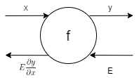 역전파의 계산 절차는 신호 $E$에 노드의 국소적 미분 $(\frac {\partial y}{\partial x})$을 곱한 후 다음 노드로 전달하는 것이다. 국소적 미분은 순전파 때의 $y=f(x)$ 계산의 미분을 구한다는 것이며, 이는 $x$에 대한 $y$의 미분 $(\frac {\partial y}{\partial x})$을 구한다는 뜻이다. 가령 $y=f(x) = x^{2}$이라면 $(\frac {\partial y}{\partial x}) = 2x$가 된다. 그리고 이 국솢거인 미분을 전달된 값에 곱해 앞쪽 노드로 전달한다. 이를 계산그래프로 나타내면
multiple_layer
import numpy as np
class multiple_layer:
    def __init__(self):
        self.x = None
        self.y = None

    def forward(self, x, y):
        self.x = x
        self.y = y
        out = x * y

        return out

    def backward(self, d_out):
        dx = d_out * self.y
        dy = d_out * self.x

        return dx, dy
apple = 100
apple_num = 2
tax = 1.1
mul_apple_layer = multiple_layer()
mul_tax_layer = multiple_layer()
apple_price = mul_apple_layer.forward(apple, apple_num)
price = mul_tax_layer.forward(apple_price, tax)
dprice = 1
dapple_price, dtax = mul_tax_layer.backward(dprice)
dapple, dapple_num = mul_apple_layer.backward(dapple_price)
dapple_price, dtax
(1.1, 200)
dapple, dapple_num
(2.2, 110.00000000000001)
add_layer
class addlayer:
    def __init__(self):
        pass

    def forward(self, x, y):
        out = x + y
        return out

    def backward(self, d_out):
        dx = d_out * 1
        dy = d_out * 1
        return dx, dy
Summary
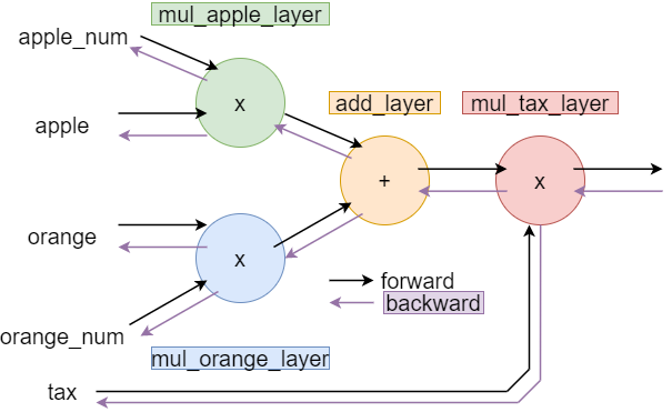
apple = 100
apple_num = 2
orange = 150
orange_num = 3
tax = 1.1

#layers
mul_apple_layer = multiple_layer()
mul_orange_layer = multiple_layer()
add_layer = addlayer()
mul_tax_layer = multiple_layer()

#forward
apple_price = mul_apple_layer.forward(apple, apple_num)
orange_price = mul_orange_layer.forward(orange, orange_num)
all_price = add_layer.forward(apple_price, orange_price)
price = mul_tax_layer.forward(all_price, tax)

#backward
d_price = 1
d_all_price, d_tax = mul_tax_layer.backward(d_price)
d_apple_price, d_orange_price = add_layer.backward(d_all_price)
d_oragne, d_orange_num = mul_orange_layer.backward(d_orange_price)
d_apple, d_apple_num = mul_apple_layer.backward(d_all_price)

print(price)
print(dapple_num, '/',d_apple, '/',d_oragne, '/',d_orange_num, '/',d_tax)
715.0000000000001
110.00000000000001 / 2.2 / 3.3000000000000003 / 165.0 / 650
Activation Function
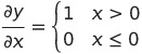
ReLU
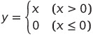
식 y 에 대한 미분은
class ReLU:
    def __init__(self):
        self.mask = None

    def forward(self, x):
        self.mask = (x <= 0)
        out = x.copy()
        out[self.mask] = 0

        return out

    def backward(self, d_out):
        d_out[self.mask] = 0
        d_x = d_out

        return d_x
x = np.array([[1.0, -0.5], [-2.0, 3.0]])
x
array([[ 1. , -0.5],
       [-2. ,  3. ]])
mask = (x <= 0)
print(mask)
[[False  True]
 [ True False]]
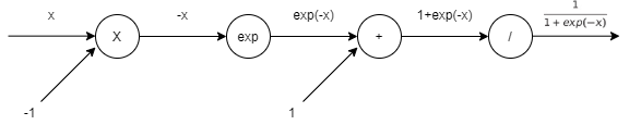
Sigmoid
$ y = \frac{1}{1+exp(-x)}$
sigmoid 계층의 순전파를 계산 그래프로 나타내면
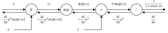
역전파 단계
1단계
’/’ 노드, $y=\frac{1}{x}$을 미분하면
$ \frac{\partial y}{\partial x} = -\frac{1}{x^{2}} = -y^{2}$
2단계
’+’노드는 상류의 값을 여과 없이 하류로 내보낸다.
3단계
‘exp’ 노드는 $y=exp(x)$ 연산을 수행하며, 미분은 $\frac{\partial y}{\partial x} = exp(x)$
4단계
‘X’노드는 순전파 때의 값을 서로 바꿔 곱한다.
모든 단계를 계산그래프로 나타내면
 간소하게 나타내면
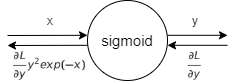
$\frac{\partial L}{\partial y}y^{2}exp(-x)$를 정리하면
$\frac{\partial L}{\partial y}y^{2}exp(-x) = \frac{\partial L}{\partial y} \frac{1}{(1+exp(-x))^{2}} exp(-x) = \frac{\partial L}{\partial y} \frac{1}{1+exp(-x)} \frac{exp(-x)}{1+exp(-x)} = \frac{\partial L}{\partial y}y(1-y)$
Sigmoid 계층의 역전파는 순전파의 출력(y)만으로도 계산할 수 있다.
class Sigmoid:
    def __init__(self):
        self.out = None

    def forward(self, x):
        out = 1 / (1 + np.exp(-x))
        self.out = out

        return out

    def backward(self, d_out):
        d_x = d_out * (1.0 - self.out) * self.out
        return d_x
참고 : 사이토 고키, 『DeepLearning from Scratch』, 한빛미디어(2020), p147-170