Time Series Analysis - Time Series with Pandas
Time Series with Pandas
from datetime import datetime
my_year = 2020
my_month = 1
my_day = 2
my_hour = 13
my_min = 30
my_sec = 15
my_date = datetime(my_year, my_month, my_day)
my_date
datetime.datetime(2020, 1, 2, 0, 0)
my_date_time = datetime(my_year, my_month, my_day, my_hour, my_min,my_sec)
my_date_time
datetime.datetime(2020, 1, 2, 13, 30, 15)
my_date_time.day
2
import numpy as np
np.array(['2020-03-15','2020-03-16','2020-03-17'], dtype = 'datetime64[D]')
array(['2020-03-15', '2020-03-16', '2020-03-17'], dtype='datetime64[D]')
np.arange('2018-06-01','2018-07-23',7, dtype = 'datetime64[D]')
array(['2018-06-01', '2018-06-08', '2018-06-15', '2018-06-22',
       '2018-06-29', '2018-07-06', '2018-07-13', '2018-07-20'],
      dtype='datetime64[D]')
import pandas as pd
pd.date_range('2020-01-01',periods=10, freq='D')
DatetimeIndex(['2020-01-01', '2020-01-02', '2020-01-03', '2020-01-04',
               '2020-01-05', '2020-01-06', '2020-01-07', '2020-01-08',
               '2020-01-09', '2020-01-10'],
              dtype='datetime64[ns]', freq='D')
pd.date_range('Jan 01, 2018',periods=10, freq='D')
DatetimeIndex(['2018-01-01', '2018-01-02', '2018-01-03', '2018-01-04',
               '2018-01-05', '2018-01-06', '2018-01-07', '2018-01-08',
               '2018-01-09', '2018-01-10'],
              dtype='datetime64[ns]', freq='D')
pd.to_datetime(['1/2/2018', 'Jan 03, 2018'])
DatetimeIndex(['2018-01-02', '2018-01-03'], dtype='datetime64[ns]', freq=None)
pd.to_datetime(['1/2/2018', '3/1/2018'], format='%d/%m/%Y')
DatetimeIndex(['2018-02-01', '2018-01-03'], dtype='datetime64[ns]', freq=None)
pd.to_datetime(['1--2--2018', '3--1--2018'], format='%d--%m--%Y')
DatetimeIndex(['2018-02-01', '2018-01-03'], dtype='datetime64[ns]', freq=None)
pd.to_datetime(['1#2#2018', '3#1#2018'], format='%d#%m#%Y')
DatetimeIndex(['2018-02-01', '2018-01-03'], dtype='datetime64[ns]', freq=None)
data = np.random.randn(3,2)
cols = ['A','B']
print(data)
[[-1.13254154  1.48492529]
 [ 1.58659165  0.12557822]
 [ 0.47964139  0.28469417]]
idx = pd.date_range('2020-01-01', periods=3, freq='D')

df = pd.DataFrame(data, columns = cols, index = idx)
df
| A | B | |
|---|---|---|
| 2020-01-01 | -1.132542 | 1.484925 |
| 2020-01-02 | 1.586592 | 0.125578 |
| 2020-01-03 | 0.479641 | 0.284694 |
df.index
DatetimeIndex(['2020-01-01', '2020-01-02', '2020-01-03'], dtype='datetime64[ns]', freq='D')
df.index.max()
Timestamp('2020-01-03 00:00:00', freq='D')
df.index.argmax()
2
df.index.min()
Timestamp('2020-01-01 00:00:00', freq='D')
df.index.argmin()
0
Time Resampling
df = pd.read_csv('Data/starbucks.csv',index_col='Date',parse_dates=True)
df.index
DatetimeIndex(['2015-01-02', '2015-01-05', '2015-01-06', '2015-01-07',
               '2015-01-08', '2015-01-09', '2015-01-12', '2015-01-13',
               '2015-01-14', '2015-01-15',
               ...
               '2018-12-17', '2018-12-18', '2018-12-19', '2018-12-20',
               '2018-12-21', '2018-12-24', '2018-12-26', '2018-12-27',
               '2018-12-28', '2018-12-31'],
              dtype='datetime64[ns]', name='Date', length=1006, freq=None)
# daily to yearly
df.resample(rule = 'A').mean()
| Close | Volume | |
|---|---|---|
| Date | ||
| 2015-12-31 | 50.078100 | 8.649190e+06 |
| 2016-12-31 | 53.891732 | 9.300633e+06 |
| 2017-12-31 | 55.457310 | 9.296078e+06 |
| 2018-12-31 | 56.870005 | 1.122883e+07 |
def first_day(entry):

    # IS THERE AN ENTRY??
    if len(entry):
        # IF SO, RETURN FIRST ENTRY
        return entry[0]
df.resample(rule='A').apply(first_day)
| Close | Volume | |
|---|---|---|
| Date | ||
| 2015-12-31 | 38.0061 | 6906098 |
| 2016-12-31 | 55.0780 | 13521544 |
| 2017-12-31 | 53.1100 | 7809307 |
| 2018-12-31 | 56.3243 | 7215978 |
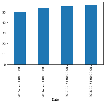
df['Close'].resample('A').mean().plot.bar()
<AxesSubplot:xlabel='Date'>
Time Shifting
df
| Close | Volume | |
|---|---|---|
| Date | ||
| 2015-01-02 | 38.0061 | 6906098 |
| 2015-01-05 | 37.2781 | 11623796 |
| 2015-01-06 | 36.9748 | 7664340 |
| 2015-01-07 | 37.8848 | 9732554 |
| 2015-01-08 | 38.4961 | 13170548 |
| ... | ... | ... |
| 2018-12-24 | 60.5600 | 6323252 |
| 2018-12-26 | 63.0800 | 16646238 |
| 2018-12-27 | 63.2000 | 11308081 |
| 2018-12-28 | 63.3900 | 7712127 |
| 2018-12-31 | 64.4000 | 7690183 |
1006 rows × 2 columns
df.tail()
| Close | Volume | |
|---|---|---|
| Date | ||
| 2018-12-24 | 60.56 | 6323252 |
| 2018-12-26 | 63.08 | 16646238 |
| 2018-12-27 | 63.20 | 11308081 |
| 2018-12-28 | 63.39 | 7712127 |
| 2018-12-31 | 64.40 | 7690183 |
df.shift(1).tail()
| Close | Volume | |
|---|---|---|
| Date | ||
| 2018-12-24 | 61.39 | 23524888.0 |
| 2018-12-26 | 60.56 | 6323252.0 |
| 2018-12-27 | 63.08 | 16646238.0 |
| 2018-12-28 | 63.20 | 11308081.0 |
| 2018-12-31 | 63.39 | 7712127.0 |
df.shift(periods=1, freq='M').head()
| Close | Volume | |
|---|---|---|
| Date | ||
| 2015-01-31 | 38.0061 | 6906098 |
| 2015-01-31 | 37.2781 | 11623796 |
| 2015-01-31 | 36.9748 | 7664340 |
| 2015-01-31 | 37.8848 | 9732554 |
| 2015-01-31 | 38.4961 | 13170548 |
df.head()
| Close | Volume | |
|---|---|---|
| Date | ||
| 2015-01-02 | 38.0061 | 6906098 |
| 2015-01-05 | 37.2781 | 11623796 |
| 2015-01-06 | 36.9748 | 7664340 |
| 2015-01-07 | 37.8848 | 9732554 |
| 2015-01-08 | 38.4961 | 13170548 |
Rolling and Expanding
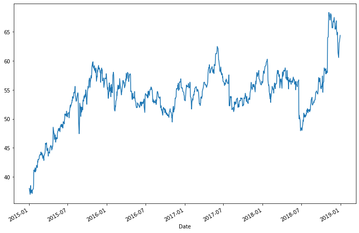
df['Close'].plot(figsize=(12,8))
<AxesSubplot:xlabel='Date'>
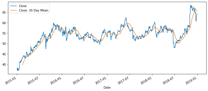
df['Close'].plot(figsize=(12,5), legend=True)
df.rolling(window=30).mean()['Close'].plot(legend=True)
<AxesSubplot:xlabel='Date'>
df['Close: 30 Day Mean'] = df['Close'].rolling(window=30).mean()
df.head()
| Close | Volume | Close: 30 Day Mean | |
|---|---|---|---|
| Date | |||
| 2015-01-02 | 38.0061 | 6906098 | NaN |
| 2015-01-05 | 37.2781 | 11623796 | NaN |
| 2015-01-06 | 36.9748 | 7664340 | NaN |
| 2015-01-07 | 37.8848 | 9732554 | NaN |
| 2015-01-08 | 38.4961 | 13170548 | NaN |
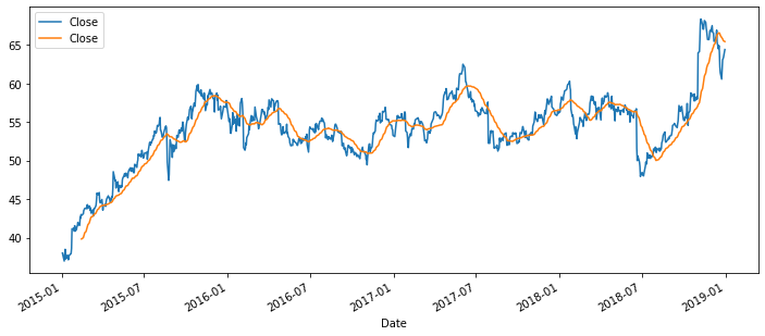
df[['Close', 'Close: 30 Day Mean']].plot(figsize=(12,5))
<AxesSubplot:xlabel='Date'>
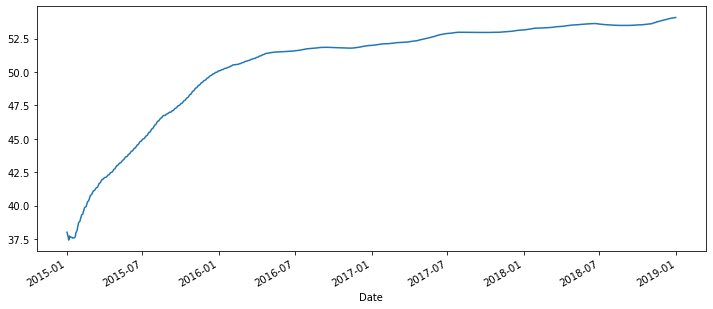
df['Close'].expanding().mean().plot(figsize=(12,5))
<AxesSubplot:xlabel='Date'>
Visualizing Time Series Data with Pandas
df.index = pd.to_datetime(df.index)
df.index
DatetimeIndex(['2015-01-02', '2015-01-05', '2015-01-06', '2015-01-07',
               '2015-01-08', '2015-01-09', '2015-01-12', '2015-01-13',
               '2015-01-14', '2015-01-15',
               ...
               '2018-12-17', '2018-12-18', '2018-12-19', '2018-12-20',
               '2018-12-21', '2018-12-24', '2018-12-26', '2018-12-27',
               '2018-12-28', '2018-12-31'],
              dtype='datetime64[ns]', name='Date', length=1006, freq=None)
df.columns
Index(['Close', 'Volume', 'Close: 30 Day Mean'], dtype='object')
df.drop(['Close: 30 Day Mean'], axis=1, inplace=True)
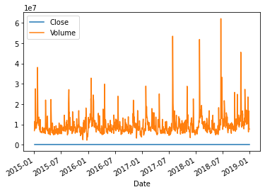
df.plot()
<AxesSubplot:xlabel='Date'>
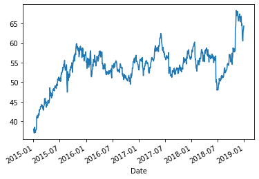
df['Close'].plot()
<AxesSubplot:xlabel='Date'>
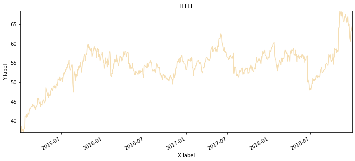
title = 'TITLE'
ylabel = 'Y label'
xlabel = 'X label'
ax = df['Close'].plot(figsize=(12,5), title=title, color='wheat')
ax.autoscale(axis='both', tight = True)
ax.set(xlabel=xlabel, ylabel=ylabel)
[Text(0.5, 0, 'X label'), Text(0, 0.5, 'Y label')]
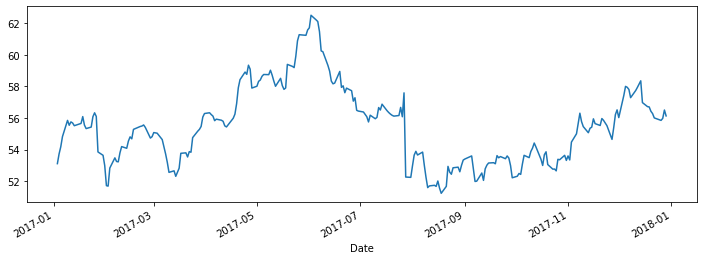
df['Close']['2017-01-01':'2017-12-31'].plot(figsize=(12,4))
<AxesSubplot:xlabel='Date'>
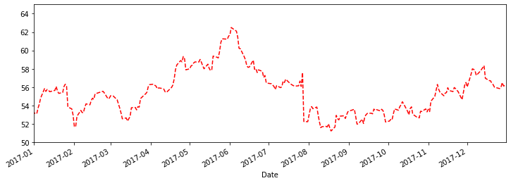
df['Close'].plot(figsize=(12,4), xlim=['2017-01-01','2017-12-31'], ylim=[50,65]
                , ls='--', c='red')
<AxesSubplot:xlabel='Date'>
from matplotlib import dates
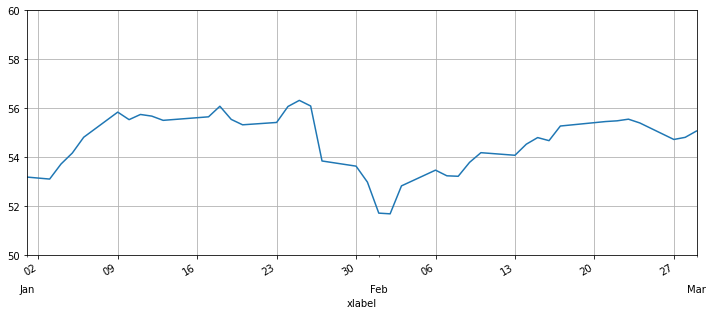
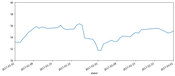
ax = df['Close'].plot(xlim=['2017-01-01','2017-03-01'], ylim=[50,60],figsize=(12,5))
ax.set(xlabel='xlabel')
[Text(0.5, 0, 'xlabel')]
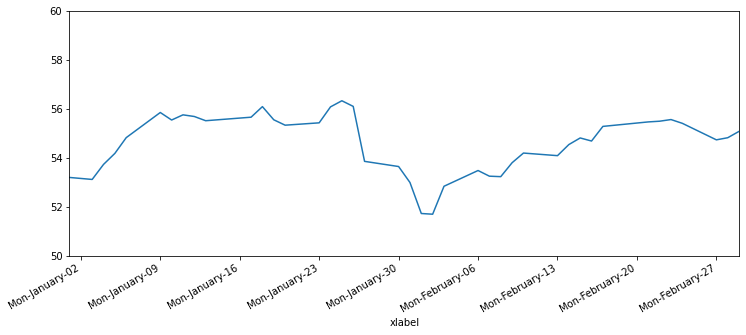
ax = df['Close'].plot(xlim=['2017-01-01','2017-03-01'], ylim=[50,60],figsize=(12,5))
ax.set(xlabel='xlabel')
ax.xaxis.set_major_locator(dates.WeekdayLocator(byweekday=0))
ax.xaxis.set_major_formatter(dates.DateFormatter('%a-%B-%d'))
ax = df['Close'].plot(xlim=['2017-01-01','2017-03-01'], ylim=[50,60],figsize=(12,5))
ax.set(xlabel='xlabel')
ax.xaxis.set_major_locator(dates.WeekdayLocator(byweekday=0))
ax.xaxis.set_major_formatter(dates.DateFormatter('%d'))

ax.xaxis.set_minor_locator(dates.MonthLocator())
ax.xaxis.set_minor_formatter(dates.DateFormatter('\n\n%b'))

ax.yaxis.grid(True)
ax.xaxis.grid(True)