Time Series Analysis - Time Series Analysis with Statsmodels
Time Series Analysis with Statsmodels
import numpy as np
import pandas as pd
%matplotlib inline

import matplotlib.pyplot as plt
df = pd.read_csv('Data/macrodata.csv', index_col = 0, parse_dates = True)
df.head()
| year | quarter | realgdp | realcons | realinv | realgovt | realdpi | cpi | m1 | tbilrate | unemp | pop | infl | realint | |
|---|---|---|---|---|---|---|---|---|---|---|---|---|---|---|
| 1959-03-31 | 1959 | 1 | 2710.349 | 1707.4 | 286.898 | 470.045 | 1886.9 | 28.98 | 139.7 | 2.82 | 5.8 | 177.146 | 0.00 | 0.00 |
| 1959-06-30 | 1959 | 2 | 2778.801 | 1733.7 | 310.859 | 481.301 | 1919.7 | 29.15 | 141.7 | 3.08 | 5.1 | 177.830 | 2.34 | 0.74 |
| 1959-09-30 | 1959 | 3 | 2775.488 | 1751.8 | 289.226 | 491.260 | 1916.4 | 29.35 | 140.5 | 3.82 | 5.3 | 178.657 | 2.74 | 1.09 |
| 1959-12-31 | 1959 | 4 | 2785.204 | 1753.7 | 299.356 | 484.052 | 1931.3 | 29.37 | 140.0 | 4.33 | 5.6 | 179.386 | 0.27 | 4.06 |
| 1960-03-31 | 1960 | 1 | 2847.699 | 1770.5 | 331.722 | 462.199 | 1955.5 | 29.54 | 139.6 | 3.50 | 5.2 | 180.007 | 2.31 | 1.19 |
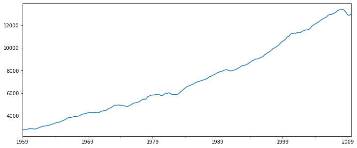
df['realgdp'].plot(figsize =(12,5))
<AxesSubplot:>
from statsmodels.tsa.filters.hp_filter import hpfilter
gdp_cycle, gdp_trend = hpfilter(df['realgdp'])
type(gdp_trend)
pandas.core.series.Series
df['trend'] = gdp_trend
df.head()
| year | quarter | realgdp | realcons | realinv | realgovt | realdpi | cpi | m1 | tbilrate | unemp | pop | infl | realint | trend | |
|---|---|---|---|---|---|---|---|---|---|---|---|---|---|---|---|
| 1959-03-31 | 1959 | 1 | 2710.349 | 1707.4 | 286.898 | 470.045 | 1886.9 | 28.98 | 139.7 | 2.82 | 5.8 | 177.146 | 0.00 | 0.00 | 2670.837085 |
| 1959-06-30 | 1959 | 2 | 2778.801 | 1733.7 | 310.859 | 481.301 | 1919.7 | 29.15 | 141.7 | 3.08 | 5.1 | 177.830 | 2.34 | 0.74 | 2698.712468 |
| 1959-09-30 | 1959 | 3 | 2775.488 | 1751.8 | 289.226 | 491.260 | 1916.4 | 29.35 | 140.5 | 3.82 | 5.3 | 178.657 | 2.74 | 1.09 | 2726.612545 |
| 1959-12-31 | 1959 | 4 | 2785.204 | 1753.7 | 299.356 | 484.052 | 1931.3 | 29.37 | 140.0 | 4.33 | 5.6 | 179.386 | 0.27 | 4.06 | 2754.612067 |
| 1960-03-31 | 1960 | 1 | 2847.699 | 1770.5 | 331.722 | 462.199 | 1955.5 | 29.54 | 139.6 | 3.50 | 5.2 | 180.007 | 2.31 | 1.19 | 2782.816333 |
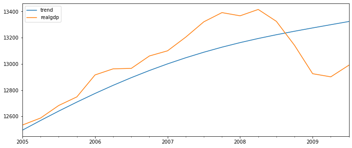
df[['trend','realgdp']]['2005-01-01':].plot(figsize = (12, 5))
<AxesSubplot:>
ETS Models
airline = pd.read_csv('Data/airline_passengers.csv', index_col = 'Month', parse_dates=True)
airline = airline.dropna()
airline.head()
| Thousands of Passengers | |
|---|---|
| Month | |
| 1949-01-01 | 112 |
| 1949-02-01 | 118 |
| 1949-03-01 | 132 |
| 1949-04-01 | 129 |
| 1949-05-01 | 121 |
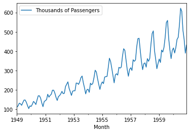
airline.plot()
<AxesSubplot:xlabel='Month'>
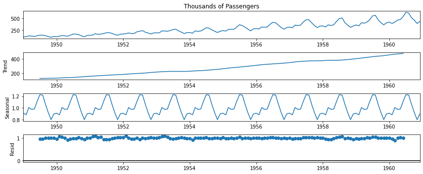
from statsmodels.tsa.seasonal import seasonal_decompose
result = seasonal_decompose(airline['Thousands of Passengers'], model='multiplicative')
from pylab import rcParams
rcParams['figure.figsize'] = 12,5

result.plot();
EWMA Models
import numpy as np
import pandas as pd
import matplotlib.pyplot as plt
%matplotlib inline
airline = pd.read_csv('Data/airline_passengers.csv', index_col="Month")
airline.dropna(inplace=True)
airline.index = pd.to_datetime(airline.index)
airline.index
DatetimeIndex(['1949-01-01', '1949-02-01', '1949-03-01', '1949-04-01',
               '1949-05-01', '1949-06-01', '1949-07-01', '1949-08-01',
               '1949-09-01', '1949-10-01',
               ...
               '1960-03-01', '1960-04-01', '1960-05-01', '1960-06-01',
               '1960-07-01', '1960-08-01', '1960-09-01', '1960-10-01',
               '1960-11-01', '1960-12-01'],
              dtype='datetime64[ns]', name='Month', length=144, freq=None)
airline.head()
| Thousands of Passengers | |
|---|---|
| Month | |
| 1949-01-01 | 112 |
| 1949-02-01 | 118 |
| 1949-03-01 | 132 |
| 1949-04-01 | 129 |
| 1949-05-01 | 121 |
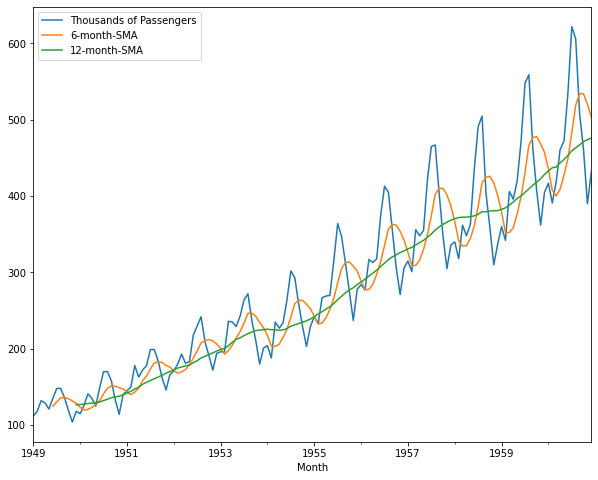
airline['6-month-SMA'] = airline['Thousands of Passengers'].rolling(window=6).mean()
airline['12-month-SMA'] = airline['Thousands of Passengers'].rolling(window=12).mean()
airline.plot(figsize = (10, 8));
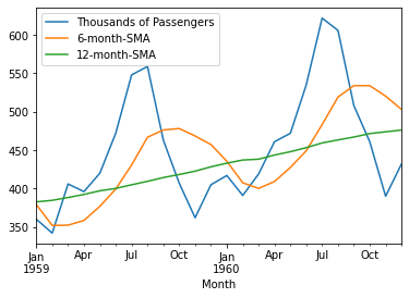
airline['1959':].plot();
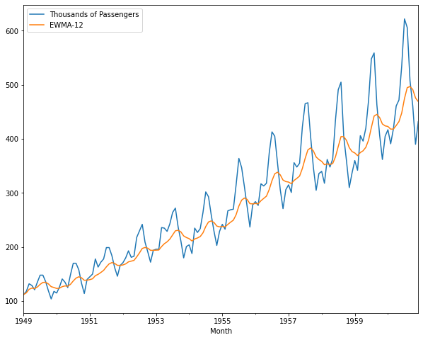
airline['EWMA-12'] = airline['Thousands of Passengers'].ewm(span = 12).mean()
airline[['Thousands of Passengers','EWMA-12']].plot(figsize = (10, 8))
<AxesSubplot:xlabel='Month'>
Holt - Winters Methods
import numpy as np
import pandas as pd
%matplotlib inline
df = pd.read_csv('Data/airline_passengers.csv', index_col = 'Month', parse_dates=True)
df = df.dropna()
df.index
DatetimeIndex(['1949-01-01', '1949-02-01', '1949-03-01', '1949-04-01',
               '1949-05-01', '1949-06-01', '1949-07-01', '1949-08-01',
               '1949-09-01', '1949-10-01',
               ...
               '1960-03-01', '1960-04-01', '1960-05-01', '1960-06-01',
               '1960-07-01', '1960-08-01', '1960-09-01', '1960-10-01',
               '1960-11-01', '1960-12-01'],
              dtype='datetime64[ns]', name='Month', length=144, freq=None)
df.index.freq = 'MS'
df.index
DatetimeIndex(['1949-01-01', '1949-02-01', '1949-03-01', '1949-04-01',
               '1949-05-01', '1949-06-01', '1949-07-01', '1949-08-01',
               '1949-09-01', '1949-10-01',
               ...
               '1960-03-01', '1960-04-01', '1960-05-01', '1960-06-01',
               '1960-07-01', '1960-08-01', '1960-09-01', '1960-10-01',
               '1960-11-01', '1960-12-01'],
              dtype='datetime64[ns]', name='Month', length=144, freq='MS')
df.head()
| Thousands of Passengers | |
|---|---|
| Month | |
| 1949-01-01 | 112 |
| 1949-02-01 | 118 |
| 1949-03-01 | 132 |
| 1949-04-01 | 129 |
| 1949-05-01 | 121 |
from statsmodels.tsa.holtwinters import SimpleExpSmoothing
span = 12
alpha = 2/(span+1)
df['EWMA12'] = df['Thousands of Passengers'].ewm(alpha = alpha, adjust = False).mean()
df.head()
| Thousands of Passengers | EWMA12 | |
|---|---|---|
| Month | ||
| 1949-01-01 | 112 | 112.000000 |
| 1949-02-01 | 118 | 112.923077 |
| 1949-03-01 | 132 | 115.857988 |
| 1949-04-01 | 129 | 117.879836 |
| 1949-05-01 | 121 | 118.359861 |
model = SimpleExpSmoothing(df['Thousands of Passengers'])
C:\Users\ilvna\.conda\envs\tf-2.3\lib\site-packages\statsmodels\tsa\holtwinters\model.py:429: FutureWarning: After 0.13 initialization must be handled at model creation
  FutureWarning,
fitted_model = model.fit(smoothing_level=alpha, optimized=False)
df['SES12'] = fitted_model.fittedvalues.shift(-1)
df.head()
| Thousands of Passengers | EWMA12 | SES12 | |
|---|---|---|---|
| Month | |||
| 1949-01-01 | 112 | 112.000000 | 112.000000 |
| 1949-02-01 | 118 | 112.923077 | 112.923077 |
| 1949-03-01 | 132 | 115.857988 | 115.857988 |
| 1949-04-01 | 129 | 117.879836 | 117.879836 |
| 1949-05-01 | 121 | 118.359861 | 118.359861 |
# df['SES12'] = SimpleExpSmoothing(df['Thousands of Passengers']).fit(smoothing_level=alpha, optimized=False).fittedvalues.shift(-1)
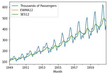
from statsmodels.tsa.holtwinters import ExponentialSmoothing
df.plot()
<AxesSubplot:xlabel='Month'>
df['DES_add_12'] = ExponentialSmoothing(df['Thousands of Passengers'],trend='add').fit().fittedvalues.shift(-1)
C:\Users\ilvna\.conda\envs\tf-2.3\lib\site-packages\statsmodels\tsa\holtwinters\model.py:429: FutureWarning: After 0.13 initialization must be handled at model creation
  FutureWarning,
df['DES_mul_12'] = ExponentialSmoothing(df['Thousands of Passengers'],trend='mul').fit().fittedvalues.shift(-1)
C:\Users\ilvna\.conda\envs\tf-2.3\lib\site-packages\statsmodels\tsa\holtwinters\model.py:429: FutureWarning: After 0.13 initialization must be handled at model creation
  FutureWarning,
df.head()
| Thousands of Passengers | EWMA12 | SES12 | DES_add_12 | DES_mul_12 | |
|---|---|---|---|---|---|
| Month | |||||
| 1949-01-01 | 112 | 112.000000 | 112.000000 | 114.221156 | 112.688538 |
| 1949-02-01 | 118 | 112.923077 | 112.923077 | 120.175837 | 118.725424 |
| 1949-03-01 | 132 | 115.857988 | 115.857988 | 134.115056 | 132.811491 |
| 1949-04-01 | 129 | 117.879836 | 117.879836 | 131.244976 | 129.793048 |
| 1949-05-01 | 121 | 118.359861 | 118.359861 | 123.283465 | 121.743867 |
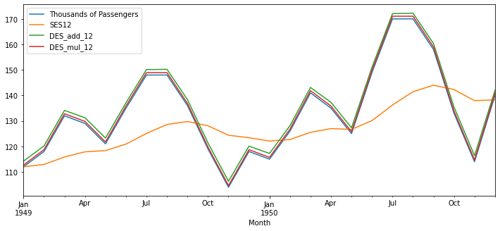
df[['Thousands of Passengers', 'SES12', 'DES_add_12','DES_mul_12']].iloc[:24].plot(figsize=(12,5))
<AxesSubplot:xlabel='Month'>
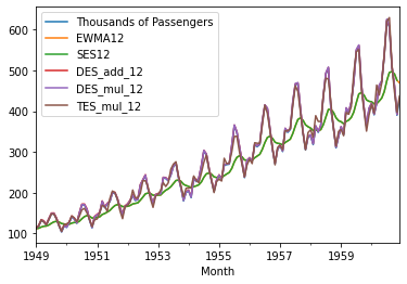
df['TES_mul_12']=ExponentialSmoothing(df['Thousands of Passengers'],trend='mul',seasonal='mul',seasonal_periods=12).fit().fittedvalues
C:\Users\ilvna\.conda\envs\tf-2.3\lib\site-packages\statsmodels\tsa\holtwinters\model.py:429: FutureWarning: After 0.13 initialization must be handled at model creation
  FutureWarning,
C:\Users\ilvna\.conda\envs\tf-2.3\lib\site-packages\statsmodels\tsa\holtwinters\model.py:80: RuntimeWarning: overflow encountered in matmul
  return err.T @ err
df.plot()
<AxesSubplot:xlabel='Month'>
df.columns
Index(['Thousands of Passengers', 'EWMA12', 'SES12', 'DES_add_12',
       'DES_mul_12', 'TES_mul_12'],
      dtype='object')
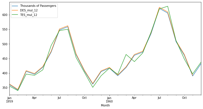
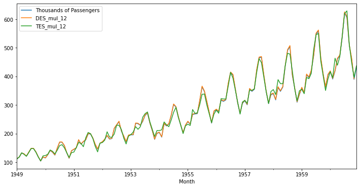
df[['Thousands of Passengers', 'DES_mul_12', 'TES_mul_12']].plot(figsize=(12,6))
<AxesSubplot:xlabel='Month'>
df[['Thousands of Passengers', 'DES_mul_12', 'TES_mul_12']].iloc[-24:].plot(figsize=(12,6))
<AxesSubplot:xlabel='Month'>