Time Series Analysis - ARIMA
ARIMA Theory
import pandas as pd
import numpy as np
%matplotlib inline

df1 = pd.read_csv('Data/airline_passengers.csv', index_col='Month', parse_dates=True)
df1.index.freq = 'MS'

df2 = pd.read_csv('Data/DailyTotalFemaleBirths.csv', index_col='Date', parse_dates=True)
df2.index.freq = 'D'
from pmdarima import auto_arima
import warnings
warnings.filterwarnings('ignore')
stepwise_fit = auto_arima(df2['Births'], start_p=0, start_q=0, max_p=6, max_q=3, seasonal=False, trace=True)
Performing stepwise search to minimize aic
 ARIMA(0,1,0)(0,0,0)[0] intercept   : AIC=2650.760, Time=0.01 sec
 ARIMA(1,1,0)(0,0,0)[0] intercept   : AIC=2565.234, Time=0.04 sec
 ARIMA(0,1,1)(0,0,0)[0] intercept   : AIC=2463.584, Time=0.07 sec
 ARIMA(0,1,0)(0,0,0)[0]             : AIC=2648.768, Time=0.01 sec
 ARIMA(1,1,1)(0,0,0)[0] intercept   : AIC=2460.154, Time=0.13 sec
 ARIMA(2,1,1)(0,0,0)[0] intercept   : AIC=2461.271, Time=0.18 sec
 ARIMA(1,1,2)(0,0,0)[0] intercept   : AIC=inf, Time=0.34 sec
 ARIMA(0,1,2)(0,0,0)[0] intercept   : AIC=2460.722, Time=0.14 sec
 ARIMA(2,1,0)(0,0,0)[0] intercept   : AIC=2536.154, Time=0.09 sec
 ARIMA(2,1,2)(0,0,0)[0] intercept   : AIC=2462.864, Time=0.44 sec
 ARIMA(1,1,1)(0,0,0)[0]             : AIC=2459.074, Time=0.05 sec
 ARIMA(0,1,1)(0,0,0)[0]             : AIC=2462.221, Time=0.02 sec
 ARIMA(1,1,0)(0,0,0)[0]             : AIC=2563.261, Time=0.02 sec
 ARIMA(2,1,1)(0,0,0)[0]             : AIC=2460.367, Time=0.08 sec
 ARIMA(1,1,2)(0,0,0)[0]             : AIC=2460.427, Time=0.13 sec
 ARIMA(0,1,2)(0,0,0)[0]             : AIC=2459.571, Time=0.04 sec
 ARIMA(2,1,0)(0,0,0)[0]             : AIC=2534.205, Time=0.03 sec
 ARIMA(2,1,2)(0,0,0)[0]             : AIC=2462.366, Time=0.21 sec

Best model:  ARIMA(1,1,1)(0,0,0)[0]
Total fit time: 2.041 seconds
stepwise_fit.summary()
| Dep. Variable: | y | No. Observations: | 365 |
|---|---|---|---|
| Model: | SARIMAX(1, 1, 1) | Log Likelihood | -1226.537 |
| Date: | Fri, 20 Nov 2020 | AIC | 2459.074 |
| Time: | 14:27:52 | BIC | 2470.766 |
| Sample: | 0 | HQIC | 2463.721 |
| - 365 | |||
| Covariance Type: | opg |
| coef | std err | z | P>|z| | [0.025 | 0.975] | |
|---|---|---|---|---|---|---|
| ar.L1 | 0.1252 | 0.060 | 2.097 | 0.036 | 0.008 | 0.242 |
| ma.L1 | -0.9624 | 0.017 | -56.429 | 0.000 | -0.996 | -0.929 |
| sigma2 | 49.1512 | 3.250 | 15.122 | 0.000 | 42.781 | 55.522 |
| Ljung-Box (Q): | 37.21 | Jarque-Bera (JB): | 25.33 |
|---|---|---|---|
| Prob(Q): | 0.60 | Prob(JB): | 0.00 |
| Heteroskedasticity (H): | 0.96 | Skew: | 0.57 |
| Prob(H) (two-sided): | 0.81 | Kurtosis: | 3.60 |
Warnings:
[1] Covariance matrix calculated using the outer product of gradients (complex-step).
stepwise_fit = auto_arima(df1['Thousands of Passengers'], start_p=0, start_q=0, max_p=4,max_q=4, seasonal=True, trace=True, m=12)
Performing stepwise search to minimize aic
 ARIMA(0,1,0)(1,1,1)[12]             : AIC=1032.128, Time=0.14 sec
 ARIMA(0,1,0)(0,1,0)[12]             : AIC=1031.508, Time=0.01 sec
 ARIMA(1,1,0)(1,1,0)[12]             : AIC=1020.393, Time=0.06 sec
 ARIMA(0,1,1)(0,1,1)[12]             : AIC=1021.003, Time=0.10 sec
 ARIMA(1,1,0)(0,1,0)[12]             : AIC=1020.393, Time=0.02 sec
 ARIMA(1,1,0)(2,1,0)[12]             : AIC=1019.239, Time=0.19 sec
 ARIMA(1,1,0)(2,1,1)[12]             : AIC=inf, Time=1.14 sec
 ARIMA(1,1,0)(1,1,1)[12]             : AIC=1020.493, Time=0.21 sec
 ARIMA(0,1,0)(2,1,0)[12]             : AIC=1032.120, Time=0.12 sec
 ARIMA(2,1,0)(2,1,0)[12]             : AIC=1021.120, Time=0.23 sec
 ARIMA(1,1,1)(2,1,0)[12]             : AIC=1021.032, Time=0.32 sec
 ARIMA(0,1,1)(2,1,0)[12]             : AIC=1019.178, Time=0.18 sec
 ARIMA(0,1,1)(1,1,0)[12]             : AIC=1020.425, Time=0.07 sec
 ARIMA(0,1,1)(2,1,1)[12]             : AIC=inf, Time=1.11 sec
 ARIMA(0,1,1)(1,1,1)[12]             : AIC=1020.327, Time=0.25 sec
 ARIMA(0,1,2)(2,1,0)[12]             : AIC=1021.148, Time=0.20 sec
 ARIMA(1,1,2)(2,1,0)[12]             : AIC=1022.805, Time=0.38 sec
 ARIMA(0,1,1)(2,1,0)[12] intercept   : AIC=1021.017, Time=0.34 sec

Best model:  ARIMA(0,1,1)(2,1,0)[12]
Total fit time: 5.096 seconds
stepwise_fit.summary()
| Dep. Variable: | y | No. Observations: | 144 |
|---|---|---|---|
| Model: | SARIMAX(0, 1, 1)x(2, 1, [], 12) | Log Likelihood | -505.589 |
| Date: | Fri, 20 Nov 2020 | AIC | 1019.178 |
| Time: | 14:27:58 | BIC | 1030.679 |
| Sample: | 0 | HQIC | 1023.851 |
| - 144 | |||
| Covariance Type: | opg |
| coef | std err | z | P>|z| | [0.025 | 0.975] | |
|---|---|---|---|---|---|---|
| ma.L1 | -0.3634 | 0.074 | -4.945 | 0.000 | -0.508 | -0.219 |
| ar.S.L12 | -0.1239 | 0.090 | -1.372 | 0.170 | -0.301 | 0.053 |
| ar.S.L24 | 0.1911 | 0.107 | 1.783 | 0.075 | -0.019 | 0.401 |
| sigma2 | 130.4480 | 15.527 | 8.402 | 0.000 | 100.016 | 160.880 |
| Ljung-Box (Q): | 53.71 | Jarque-Bera (JB): | 4.59 |
|---|---|---|---|
| Prob(Q): | 0.07 | Prob(JB): | 0.10 |
| Heteroskedasticity (H): | 2.70 | Skew: | 0.15 |
| Prob(H) (two-sided): | 0.00 | Kurtosis: | 3.87 |
Warnings:
[1] Covariance matrix calculated using the outer product of gradients (complex-step).
ARMA and ARIMA
import pandas as pd
import numpy as np
%matplotlib inline

import warnings
warnings.filterwarnings('ignore')
from statsmodels.tsa.arima_model import ARMA, ARIMA, ARMAResults, ARIMAResults
from statsmodels.tsa.statespace.sarimax import SARIMAX, SARIMAXResults
from statsmodels.graphics.tsaplots import plot_acf, plot_pacf
from pmdarima.arima import auto_arima
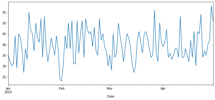
df1 = pd.read_csv('Data/DailyTotalFemaleBirths.csv', index_col='Date',parse_dates=True)
df1.index.freq = 'D'
df1 = df1[:120]
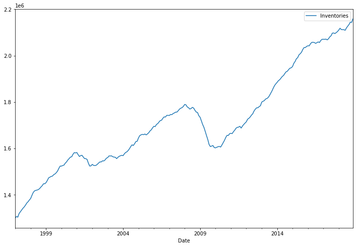
df2 = pd.read_csv('Data/TradeInventories.csv',index_col='Date',parse_dates=True)
df2.index.freq='MS'
ARMA
df1['Births'].plot(figsize=(12,5))
<AxesSubplot:xlabel='Date'>
from statsmodels.tsa.stattools import adfuller

def adf_test(series, title=''):
    """
    Pass in a time series and an optional title, returns an ADF report
    """
    print(f'Augmented Dickey-Fuller Test: {title}')
    result = adfuller(series.dropna(), autolag = 'AIC')

    labels = ['ADF test statistic', 'p-value', '# lags used', '# obervations']
    out = pd.Series(result[0:4], index = labels)

    for key, val in result[4].items():
        out[f'critical value ({key})'] = val

    print(out.to_string())

    if result[1] <= 0.05:
        print('Strong evidence against the null hypothesis')
        print('Reject the null hypothesis')
        print('Data has no unit root and is stationary')
    else:
        print('Weak evidence against the null hypothesis')
        print('Fail to reject the null hypothesis')
        print('Data has a unit root and is non-stationary')
adf_test(df1['Births'])
Augmented Dickey-Fuller Test:
ADF test statistic     -9.855384e+00
p-value                 4.373545e-17
# lags used             0.000000e+00
# obervations           1.190000e+02
critical value (1%)    -3.486535e+00
critical value (5%)    -2.886151e+00
critical value (10%)   -2.579896e+00
Strong evidence against the null hypothesis
Reject the null hypothesis
Data has no unit root and is stationary
auto_arima(df1['Births'], seasonal=False, trace=True).summary()
Performing stepwise search to minimize aic
 ARIMA(2,0,2)(0,0,0)[0]             : AIC=inf, Time=0.14 sec
 ARIMA(0,0,0)(0,0,0)[0]             : AIC=1230.607, Time=0.00 sec
 ARIMA(1,0,0)(0,0,0)[0]             : AIC=896.926, Time=0.01 sec
 ARIMA(0,0,1)(0,0,0)[0]             : AIC=1121.103, Time=0.02 sec
 ARIMA(2,0,0)(0,0,0)[0]             : AIC=inf, Time=0.03 sec
 ARIMA(1,0,1)(0,0,0)[0]             : AIC=inf, Time=0.10 sec


C:\Users\ilvna\.conda\envs\tf-2.3\lib\site-packages\statsmodels\base\model.py:568: ConvergenceWarning: Maximum Likelihood optimization failed to converge. Check mle_retvals
  "Check mle_retvals", ConvergenceWarning)
C:\Users\ilvna\.conda\envs\tf-2.3\lib\site-packages\statsmodels\base\model.py:568: ConvergenceWarning: Maximum Likelihood optimization failed to converge. Check mle_retvals
  "Check mle_retvals", ConvergenceWarning)


 ARIMA(2,0,1)(0,0,0)[0]             : AIC=inf, Time=0.14 sec
 ARIMA(1,0,0)(0,0,0)[0] intercept   : AIC=824.647, Time=0.02 sec
 ARIMA(0,0,0)(0,0,0)[0] intercept   : AIC=823.489, Time=0.00 sec
 ARIMA(0,0,1)(0,0,0)[0] intercept   : AIC=824.747, Time=0.03 sec
 ARIMA(1,0,1)(0,0,0)[0] intercept   : AIC=826.399, Time=0.15 sec

Best model:  ARIMA(0,0,0)(0,0,0)[0] intercept
Total fit time: 0.662 seconds
| Dep. Variable: | y | No. Observations: | 120 |
|---|---|---|---|
| Model: | SARIMAX | Log Likelihood | -409.745 |
| Date: | Mon, 23 Nov 2020 | AIC | 823.489 |
| Time: | 13:58:39 | BIC | 829.064 |
| Sample: | 0 | HQIC | 825.753 |
| - 120 | |||
| Covariance Type: | opg |
| coef | std err | z | P>|z| | [0.025 | 0.975] | |
|---|---|---|---|---|---|---|
| intercept | 39.7833 | 0.687 | 57.896 | 0.000 | 38.437 | 41.130 |
| sigma2 | 54.1197 | 8.319 | 6.506 | 0.000 | 37.815 | 70.424 |
| Ljung-Box (Q): | 44.41 | Jarque-Bera (JB): | 2.69 |
|---|---|---|---|
| Prob(Q): | 0.29 | Prob(JB): | 0.26 |
| Heteroskedasticity (H): | 0.80 | Skew: | 0.26 |
| Prob(H) (two-sided): | 0.48 | Kurtosis: | 2.48 |
Warnings:
[1] Covariance matrix calculated using the outer product of gradients (complex-step).
train = df1.iloc[:90]
test = df1.iloc[90:]
model = ARMA(train['Births'], order=(2,2))
results = model.fit()
results.summary()
| Dep. Variable: | Births | No. Observations: | 90 |
|---|---|---|---|
| Model: | ARMA(2, 2) | Log Likelihood | -307.905 |
| Method: | css-mle | S.D. of innovations | 7.405 |
| Date: | Mon, 23 Nov 2020 | AIC | 627.809 |
| Time: | 13:58:39 | BIC | 642.808 |
| Sample: | 01-01-1959 | HQIC | 633.858 |
| - 03-31-1959 |
| coef | std err | z | P>|z| | [0.025 | 0.975] | |
|---|---|---|---|---|---|---|
| const | 39.7549 | 0.912 | 43.607 | 0.000 | 37.968 | 41.542 |
| ar.L1.Births | -0.1850 | 1.087 | -0.170 | 0.865 | -2.315 | 1.945 |
| ar.L2.Births | 0.4352 | 0.644 | 0.675 | 0.500 | -0.828 | 1.698 |
| ma.L1.Births | 0.2777 | 1.097 | 0.253 | 0.800 | -1.872 | 2.427 |
| ma.L2.Births | -0.3999 | 0.679 | -0.589 | 0.556 | -1.730 | 0.930 |
| Real | Imaginary | Modulus | Frequency | |
|---|---|---|---|---|
| AR.1 | -1.3181 | +0.0000j | 1.3181 | 0.5000 |
| AR.2 | 1.7433 | +0.0000j | 1.7433 | 0.0000 |
| MA.1 | -1.2718 | +0.0000j | 1.2718 | 0.5000 |
| MA.2 | 1.9662 | +0.0000j | 1.9662 | 0.0000 |
start = len(train)
end = len(train) + len(test) - 1
predictions = results.predict(start, end).rename('ARMA (2,2) Predictions')
test['Births'].plot(figsize = (12,8), legend=True)
predictions.plot(legend=True)
<AxesSubplot:xlabel='Date'>
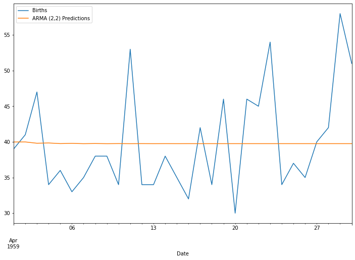
test.mean()
Births    39.833333
dtype: float64
predictions.mean()
39.777432092745876
df2.plot(figsize=(12,8))
<AxesSubplot:xlabel='Date'>
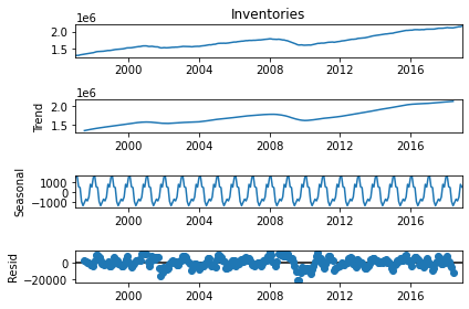
from statsmodels.tsa.seasonal import seasonal_decompose
result = seasonal_decompose(df2['Inventories'], model='add')
result.plot();
auto_arima(df2['Inventories'],seasonal=False, trace=True).summary()
Performing stepwise search to minimize aic
 ARIMA(2,1,2)(0,0,0)[0] intercept   : AIC=5373.961, Time=0.31 sec
 ARIMA(0,1,0)(0,0,0)[0] intercept   : AIC=5348.037, Time=0.04 sec
 ARIMA(1,1,0)(0,0,0)[0] intercept   : AIC=5399.843, Time=0.03 sec
 ARIMA(0,1,1)(0,0,0)[0] intercept   : AIC=5350.241, Time=0.03 sec
 ARIMA(0,1,0)(0,0,0)[0]             : AIC=5409.217, Time=0.01 sec
 ARIMA(1,1,1)(0,0,0)[0] intercept   : AIC=5378.835, Time=0.14 sec

Best model:  ARIMA(0,1,0)(0,0,0)[0] intercept
Total fit time: 0.562 seconds
| Dep. Variable: | y | No. Observations: | 264 |
|---|---|---|---|
| Model: | SARIMAX(0, 1, 0) | Log Likelihood | -2672.018 |
| Date: | Mon, 23 Nov 2020 | AIC | 5348.037 |
| Time: | 13:58:42 | BIC | 5355.181 |
| Sample: | 0 | HQIC | 5350.908 |
| - 264 | |||
| Covariance Type: | opg |
| coef | std err | z | P>|z| | [0.025 | 0.975] | |
|---|---|---|---|---|---|---|
| intercept | 3258.3802 | 470.991 | 6.918 | 0.000 | 2335.255 | 4181.506 |
| sigma2 | 3.91e+07 | 2.95e+06 | 13.250 | 0.000 | 3.33e+07 | 4.49e+07 |
| Ljung-Box (Q): | 455.75 | Jarque-Bera (JB): | 100.74 |
|---|---|---|---|
| Prob(Q): | 0.00 | Prob(JB): | 0.00 |
| Heteroskedasticity (H): | 0.86 | Skew: | -1.15 |
| Prob(H) (two-sided): | 0.48 | Kurtosis: | 4.98 |
Warnings:
[1] Covariance matrix calculated using the outer product of gradients (complex-step).
from statsmodels.tsa.statespace.tools import diff
df2['Diff_1'] = diff(df2['Inventories'], k_diff=1)
adf_test(df2['Diff_1'])
Augmented Dickey-Fuller Test:
ADF test statistic       -3.412249
p-value                   0.010548
# lags used               4.000000
# obervations           258.000000
critical value (1%)      -3.455953
critical value (5%)      -2.872809
critical value (10%)     -2.572775
Strong evidence against the null hypothesis
Reject the null hypothesis
Data has no unit root and is stationary
df2
| Inventories | Diff_1 | |
|---|---|---|
| Date | ||
| 1997-01-01 | 1301161 | NaN |
| 1997-02-01 | 1307080 | 5919.0 |
| 1997-03-01 | 1303978 | -3102.0 |
| 1997-04-01 | 1319740 | 15762.0 |
| 1997-05-01 | 1327294 | 7554.0 |
| ... | ... | ... |
| 2018-08-01 | 2127170 | 7552.0 |
| 2018-09-01 | 2134172 | 7002.0 |
| 2018-10-01 | 2144639 | 10467.0 |
| 2018-11-01 | 2143001 | -1638.0 |
| 2018-12-01 | 2158115 | 15114.0 |
264 rows × 2 columns
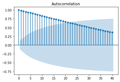
plot_acf(df2['Inventories'], lags=40);
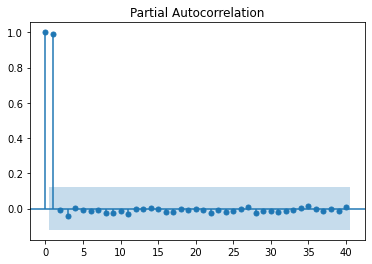
plot_pacf(df2['Inventories'], lags=40);
stepwise_fit = auto_arima(df2['Inventories'],start_p=0, start_q=0,
                          max_p=2, max_q=2, seasonal=False, trace=True)

stepwise_fit.summary()
Performing stepwise search to minimize aic
 ARIMA(0,1,0)(0,0,0)[0] intercept   : AIC=5348.037, Time=0.01 sec
 ARIMA(1,1,0)(0,0,0)[0] intercept   : AIC=5399.843, Time=0.04 sec
 ARIMA(0,1,1)(0,0,0)[0] intercept   : AIC=5350.241, Time=0.03 sec
 ARIMA(0,1,0)(0,0,0)[0]             : AIC=5409.217, Time=0.01 sec
 ARIMA(1,1,1)(0,0,0)[0] intercept   : AIC=5378.835, Time=0.14 sec

Best model:  ARIMA(0,1,0)(0,0,0)[0] intercept
Total fit time: 0.230 seconds
| Dep. Variable: | y | No. Observations: | 264 |
|---|---|---|---|
| Model: | SARIMAX(0, 1, 0) | Log Likelihood | -2672.018 |
| Date: | Fri, 20 Nov 2020 | AIC | 5348.037 |
| Time: | 14:28:12 | BIC | 5355.181 |
| Sample: | 0 | HQIC | 5350.908 |
| - 264 | |||
| Covariance Type: | opg |
| coef | std err | z | P>|z| | [0.025 | 0.975] | |
|---|---|---|---|---|---|---|
| intercept | 3258.3802 | 470.991 | 6.918 | 0.000 | 2335.255 | 4181.506 |
| sigma2 | 3.91e+07 | 2.95e+06 | 13.250 | 0.000 | 3.33e+07 | 4.49e+07 |
| Ljung-Box (Q): | 455.75 | Jarque-Bera (JB): | 100.74 |
|---|---|---|---|
| Prob(Q): | 0.00 | Prob(JB): | 0.00 |
| Heteroskedasticity (H): | 0.86 | Skew: | -1.15 |
| Prob(H) (two-sided): | 0.48 | Kurtosis: | 4.98 |
Warnings:
[1] Covariance matrix calculated using the outer product of gradients (complex-step).
train = df2.iloc[:252]
test = df2.iloc[252:]
train
| Inventories | Diff_1 | |
|---|---|---|
| Date | ||
| 1997-01-01 | 1301161 | NaN |
| 1997-02-01 | 1307080 | 5919.0 |
| 1997-03-01 | 1303978 | -3102.0 |
| 1997-04-01 | 1319740 | 15762.0 |
| 1997-05-01 | 1327294 | 7554.0 |
| ... | ... | ... |
| 2017-08-01 | 2097163 | 11650.0 |
| 2017-09-01 | 2097753 | 590.0 |
| 2017-10-01 | 2095167 | -2586.0 |
| 2017-11-01 | 2099137 | 3970.0 |
| 2017-12-01 | 2103751 | 4614.0 |
252 rows × 2 columns
model = ARIMA(train['Inventories'], order=(1,1,1))
results = model.fit()
results.summary()
| Dep. Variable: | D.Inventories | No. Observations: | 251 |
|---|---|---|---|
| Model: | ARIMA(1, 1, 1) | Log Likelihood | -2486.395 |
| Method: | css-mle | S.D. of innovations | 4845.028 |
| Date: | Thu, 15 Oct 2020 | AIC | 4980.790 |
| Time: | 13:01:13 | BIC | 4994.892 |
| Sample: | 02-01-1997 | HQIC | 4986.465 |
| - 12-01-2017 |
| coef | std err | z | P>|z| | [0.025 | 0.975] | |
|---|---|---|---|---|---|---|
| const | 3197.5697 | 1344.869 | 2.378 | 0.017 | 561.674 | 5833.465 |
| ar.L1.D.Inventories | 0.9026 | 0.039 | 23.010 | 0.000 | 0.826 | 0.979 |
| ma.L1.D.Inventories | -0.5581 | 0.079 | -7.048 | 0.000 | -0.713 | -0.403 |
| Real | Imaginary | Modulus | Frequency | |
|---|---|---|---|---|
| AR.1 | 1.1080 | +0.0000j | 1.1080 | 0.0000 |
| MA.1 | 1.7918 | +0.0000j | 1.7918 | 0.0000 |
start = len(train)
end = len(train) + len(test) - 1
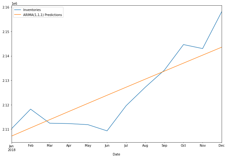
predictions = results.predict(start, end, typ='levels').rename('ARIMA(1,1,1) Predictions')
test['Inventories'].plot(figsize = (12,8), legend=True)
predictions.plot(legend=True)
<AxesSubplot:xlabel='Date'>
from statsmodels.tools.eval_measures import rmse
error = rmse(test['Inventories'], predictions)
error
7789.5973836593785
test['Inventories'].mean()
2125075.6666666665
predictions.mean()
2125465.272049339
FORECAST INTO UNKNOWN FUTURE
model = ARIMA(df2['Inventories'], order=(1,1,1))
results = model.fit()
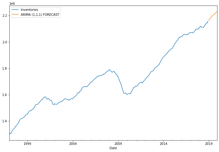
fcast = results.predict(start =len(df2),end=len(df2)+11, typ='levels').rename('ARIMA (1,1,1) FORECAST')
df2['Inventories'].plot(figsize=(12,8), legend=True)
fcast.plot(legend=True)
<AxesSubplot:xlabel='Date'>
SARIMA
import pandas as pd
import numpy as np
%matplotlib inline

import warnings
warnings.filterwarnings('ignore')
from statsmodels.tsa.statespace.sarimax import SARIMAX
from statsmodels.tsa.seasonal import seasonal_decompose
from pmdarima import auto_arima
df = pd.read_csv('Data/co2_mm_mlo.csv')
df.head()
| year | month | decimal_date | average | interpolated | |
|---|---|---|---|---|---|
| 0 | 1958 | 3 | 1958.208 | 315.71 | 315.71 |
| 1 | 1958 | 4 | 1958.292 | 317.45 | 317.45 |
| 2 | 1958 | 5 | 1958.375 | 317.50 | 317.50 |
| 3 | 1958 | 6 | 1958.458 | NaN | 317.10 |
| 4 | 1958 | 7 | 1958.542 | 315.86 | 315.86 |
# dict(year=df['year'], month=df['month'], day=1)

df['date'] = pd.to_datetime({'year':df['year'], 'month':df['month'],'day':1})
df.head()
| year | month | decimal_date | average | interpolated | date | |
|---|---|---|---|---|---|---|
| 0 | 1958 | 3 | 1958.208 | 315.71 | 315.71 | 1958-03-01 |
| 1 | 1958 | 4 | 1958.292 | 317.45 | 317.45 | 1958-04-01 |
| 2 | 1958 | 5 | 1958.375 | 317.50 | 317.50 | 1958-05-01 |
| 3 | 1958 | 6 | 1958.458 | NaN | 317.10 | 1958-06-01 |
| 4 | 1958 | 7 | 1958.542 | 315.86 | 315.86 | 1958-07-01 |
df.info()
<class 'pandas.core.frame.DataFrame'>
RangeIndex: 729 entries, 0 to 728
Data columns (total 6 columns):
 #   Column        Non-Null Count  Dtype
---  ------        --------------  -----
 0   year          729 non-null    int64
 1   month         729 non-null    int64
 2   decimal_date  729 non-null    float64
 3   average       722 non-null    float64
 4   interpolated  729 non-null    float64
 5   date          729 non-null    datetime64[ns]
dtypes: datetime64[ns](1), float64(3), int64(2)
memory usage: 34.3 KB
df = df.set_index('date')
df.head()
| year | month | decimal_date | average | interpolated | |
|---|---|---|---|---|---|
| date | |||||
| 1958-03-01 | 1958 | 3 | 1958.208 | 315.71 | 315.71 |
| 1958-04-01 | 1958 | 4 | 1958.292 | 317.45 | 317.45 |
| 1958-05-01 | 1958 | 5 | 1958.375 | 317.50 | 317.50 |
| 1958-06-01 | 1958 | 6 | 1958.458 | NaN | 317.10 |
| 1958-07-01 | 1958 | 7 | 1958.542 | 315.86 | 315.86 |
df.index.freq = 'MS'
df.head()
| year | month | decimal_date | average | interpolated | |
|---|---|---|---|---|---|
| date | |||||
| 1958-03-01 | 1958 | 3 | 1958.208 | 315.71 | 315.71 |
| 1958-04-01 | 1958 | 4 | 1958.292 | 317.45 | 317.45 |
| 1958-05-01 | 1958 | 5 | 1958.375 | 317.50 | 317.50 |
| 1958-06-01 | 1958 | 6 | 1958.458 | NaN | 317.10 |
| 1958-07-01 | 1958 | 7 | 1958.542 | 315.86 | 315.86 |
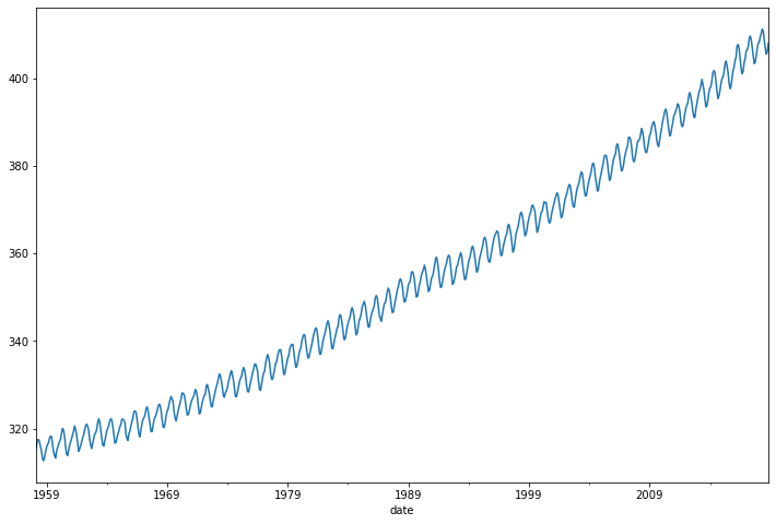
df['interpolated'].plot(figsize=(12,8))
<AxesSubplot:xlabel='date'>
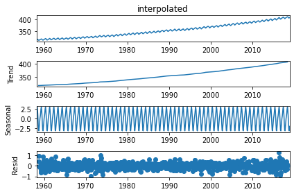
result = seasonal_decompose(df['interpolated'], model='add')
result.plot();
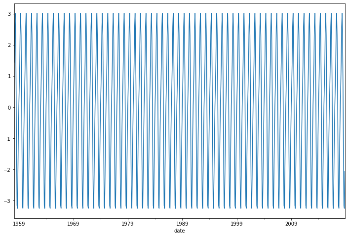
result.seasonal.plot(figsize=(12,8))
<AxesSubplot:xlabel='date'>
auto_arima(df['interpolated'],seasonal=True,m=12).summary()
| Dep. Variable: | y | No. Observations: | 729 |
|---|---|---|---|
| Model: | SARIMAX(2, 1, 1)x(1, 0, 1, 12) | Log Likelihood | -206.304 |
| Date: | Thu, 15 Oct 2020 | AIC | 424.609 |
| Time: | 13:24:28 | BIC | 452.151 |
| Sample: | 0 | HQIC | 435.236 |
| - 729 | |||
| Covariance Type: | opg |
| coef | std err | z | P>|z| | [0.025 | 0.975] | |
|---|---|---|---|---|---|---|
| ar.L1 | 0.3594 | 0.070 | 5.106 | 0.000 | 0.221 | 0.497 |
| ar.L2 | 0.0895 | 0.030 | 2.979 | 0.003 | 0.031 | 0.148 |
| ma.L1 | -0.7122 | 0.061 | -11.698 | 0.000 | -0.832 | -0.593 |
| ar.S.L12 | 0.9996 | 0.000 | 2369.802 | 0.000 | 0.999 | 1.000 |
| ma.S.L12 | -0.8653 | 0.022 | -39.952 | 0.000 | -0.908 | -0.823 |
| sigma2 | 0.0957 | 0.005 | 20.453 | 0.000 | 0.087 | 0.105 |
| Ljung-Box (Q): | 43.95 | Jarque-Bera (JB): | 4.32 |
|---|---|---|---|
| Prob(Q): | 0.31 | Prob(JB): | 0.12 |
| Heteroskedasticity (H): | 1.12 | Skew: | -0.00 |
| Prob(H) (two-sided): | 0.36 | Kurtosis: | 3.38 |
Warnings:
[1] Covariance matrix calculated using the outer product of gradients (complex-step).
len(df)
729
train = df.iloc[:717]
test = df.iloc[717:]
model = SARIMAX(train['interpolated'], order=(2,1,1),seasonal_order=(1,0,1,12))
results = model.fit()
results.summary()
| Dep. Variable: | interpolated | No. Observations: | 717 |
|---|---|---|---|
| Model: | SARIMAX(2, 1, 1)x(1, 0, 1, 12) | Log Likelihood | -201.889 |
| Date: | Thu, 15 Oct 2020 | AIC | 415.778 |
| Time: | 13:28:51 | BIC | 443.220 |
| Sample: | 03-01-1958 | HQIC | 426.375 |
| - 11-01-2017 | |||
| Covariance Type: | opg |
| coef | std err | z | P>|z| | [0.025 | 0.975] | |
|---|---|---|---|---|---|---|
| ar.L1 | 0.3458 | 0.083 | 4.154 | 0.000 | 0.183 | 0.509 |
| ar.L2 | 0.0840 | 0.039 | 2.158 | 0.031 | 0.008 | 0.160 |
| ma.L1 | -0.7032 | 0.075 | -9.432 | 0.000 | -0.849 | -0.557 |
| ar.S.L12 | 0.9996 | 0.000 | 2879.070 | 0.000 | 0.999 | 1.000 |
| ma.S.L12 | -0.8653 | 0.023 | -38.111 | 0.000 | -0.910 | -0.821 |
| sigma2 | 0.0953 | 0.005 | 20.391 | 0.000 | 0.086 | 0.104 |
| Ljung-Box (Q): | 44.35 | Jarque-Bera (JB): | 4.68 |
|---|---|---|---|
| Prob(Q): | 0.29 | Prob(JB): | 0.10 |
| Heteroskedasticity (H): | 1.14 | Skew: | 0.01 |
| Prob(H) (two-sided): | 0.31 | Kurtosis: | 3.39 |
Warnings:
[1] Covariance matrix calculated using the outer product of gradients (complex-step).
start = len(train)
end = len(train) + len(test) - 1
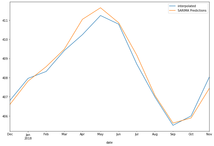
predictions = results.predict(start, end, typ='levels').rename('SARIMA Predictions')
test['interpolated'].plot(figsize=(12,8), legend=True)
predictions.plot(legend=True)
<AxesSubplot:xlabel='date'>
from statsmodels.tools.eval_measures import rmse
error = rmse(test['interpolated'], predictions)
error
0.3581857245313432
test['interpolated'].mean()
408.3333333333333
FORECAST INTO UNKWON FUTURE
model = SARIMAX(df['interpolated'], order=(2,1,1),seasonal_order=(1,0,1,12))
results = model.fit()
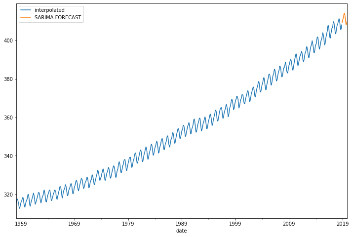
fcast = results.predict(len(df), len(df)+11, typ='levels').rename('SARIMA FORECAST')
df['interpolated'].plot(figsize=(12,8), legend=True)
fcast.plot(legend=True)
<AxesSubplot:xlabel='date'>
SARIMAX
import pandas as pd
import numpy as np
%matplotlib inline

import warnings
warnings.filterwarnings('ignore')
df=pd.read_csv('Data/RestaurantVisitors.csv',index_col='date',parse_dates=True)
df.index.freq = 'D'
df.head()
| weekday | holiday | holiday_name | rest1 | rest2 | rest3 | rest4 | total | |
|---|---|---|---|---|---|---|---|---|
| date | ||||||||
| 2016-01-01 | Friday | 1 | New Year's Day | 65.0 | 25.0 | 67.0 | 139.0 | 296.0 |
| 2016-01-02 | Saturday | 0 | na | 24.0 | 39.0 | 43.0 | 85.0 | 191.0 |
| 2016-01-03 | Sunday | 0 | na | 24.0 | 31.0 | 66.0 | 81.0 | 202.0 |
| 2016-01-04 | Monday | 0 | na | 23.0 | 18.0 | 32.0 | 32.0 | 105.0 |
| 2016-01-05 | Tuesday | 0 | na | 2.0 | 15.0 | 38.0 | 43.0 | 98.0 |
df.tail()
| weekday | holiday | holiday_name | rest1 | rest2 | rest3 | rest4 | total | |
|---|---|---|---|---|---|---|---|---|
| date | ||||||||
| 2017-05-27 | Saturday | 0 | na | NaN | NaN | NaN | NaN | NaN |
| 2017-05-28 | Sunday | 0 | na | NaN | NaN | NaN | NaN | NaN |
| 2017-05-29 | Monday | 1 | Memorial Day | NaN | NaN | NaN | NaN | NaN |
| 2017-05-30 | Tuesday | 0 | na | NaN | NaN | NaN | NaN | NaN |
| 2017-05-31 | Wednesday | 0 | na | NaN | NaN | NaN | NaN | NaN |
df1 = df.dropna()
df1.tail()
| weekday | holiday | holiday_name | rest1 | rest2 | rest3 | rest4 | total | |
|---|---|---|---|---|---|---|---|---|
| date | ||||||||
| 2017-04-18 | Tuesday | 0 | na | 30.0 | 30.0 | 13.0 | 18.0 | 91.0 |
| 2017-04-19 | Wednesday | 0 | na | 20.0 | 11.0 | 30.0 | 18.0 | 79.0 |
| 2017-04-20 | Thursday | 0 | na | 22.0 | 3.0 | 19.0 | 46.0 | 90.0 |
| 2017-04-21 | Friday | 0 | na | 38.0 | 53.0 | 36.0 | 38.0 | 165.0 |
| 2017-04-22 | Saturday | 0 | na | 97.0 | 20.0 | 50.0 | 59.0 | 226.0 |
df1.columns
Index(['weekday', 'holiday', 'holiday_name', 'rest1', 'rest2', 'rest3',
       'rest4', 'total'],
      dtype='object')
cols = ['rest1', 'rest2', 'rest3',
       'rest4', 'total']
for column in cols:
    df1[column] = df1[column].astype(int)
df1.head()
| weekday | holiday | holiday_name | rest1 | rest2 | rest3 | rest4 | total | |
|---|---|---|---|---|---|---|---|---|
| date | ||||||||
| 2016-01-01 | Friday | 1 | New Year's Day | 65 | 25 | 67 | 139 | 296 |
| 2016-01-02 | Saturday | 0 | na | 24 | 39 | 43 | 85 | 191 |
| 2016-01-03 | Sunday | 0 | na | 24 | 31 | 66 | 81 | 202 |
| 2016-01-04 | Monday | 0 | na | 23 | 18 | 32 | 32 | 105 |
| 2016-01-05 | Tuesday | 0 | na | 2 | 15 | 38 | 43 | 98 |
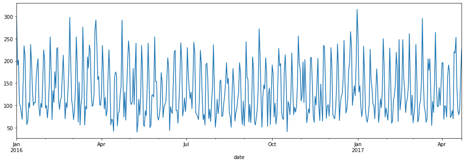
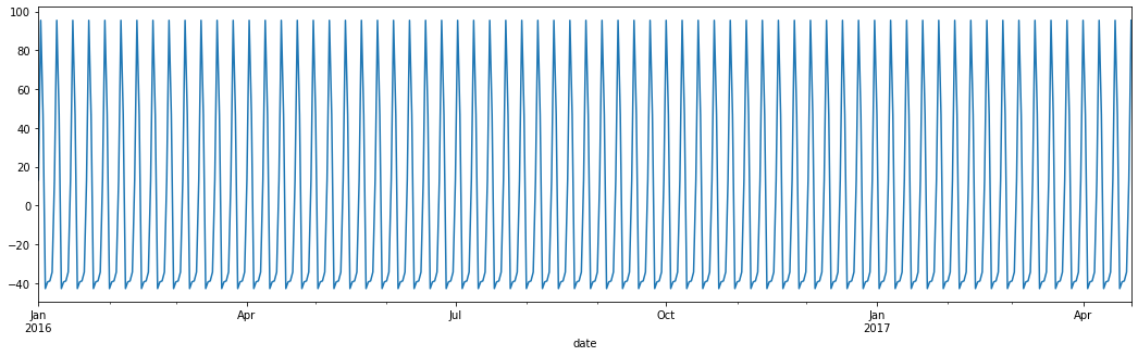
df1['total'].plot(figsize=(16,5))
<AxesSubplot:xlabel='date'>
df1.query('holiday==1').index
DatetimeIndex(['2016-01-01', '2016-01-18', '2016-02-02', '2016-02-14',
               '2016-02-15', '2016-03-17', '2016-03-25', '2016-03-27',
               '2016-03-28', '2016-05-05', '2016-05-08', '2016-05-30',
               '2016-06-19', '2016-07-04', '2016-09-05', '2016-10-10',
               '2016-10-31', '2016-11-11', '2016-11-24', '2016-11-25',
               '2016-12-24', '2016-12-25', '2016-12-31', '2017-01-01',
               '2017-01-16', '2017-02-02', '2017-02-14', '2017-02-20',
               '2017-03-17', '2017-04-14', '2017-04-16', '2017-04-17'],
              dtype='datetime64[ns]', name='date', freq=None)
df1[df1['holiday']==1].index
DatetimeIndex(['2016-01-01', '2016-01-18', '2016-02-02', '2016-02-14',
               '2016-02-15', '2016-03-17', '2016-03-25', '2016-03-27',
               '2016-03-28', '2016-05-05', '2016-05-08', '2016-05-30',
               '2016-06-19', '2016-07-04', '2016-09-05', '2016-10-10',
               '2016-10-31', '2016-11-11', '2016-11-24', '2016-11-25',
               '2016-12-24', '2016-12-25', '2016-12-31', '2017-01-01',
               '2017-01-16', '2017-02-02', '2017-02-14', '2017-02-20',
               '2017-03-17', '2017-04-14', '2017-04-16', '2017-04-17'],
              dtype='datetime64[ns]', name='date', freq=None)
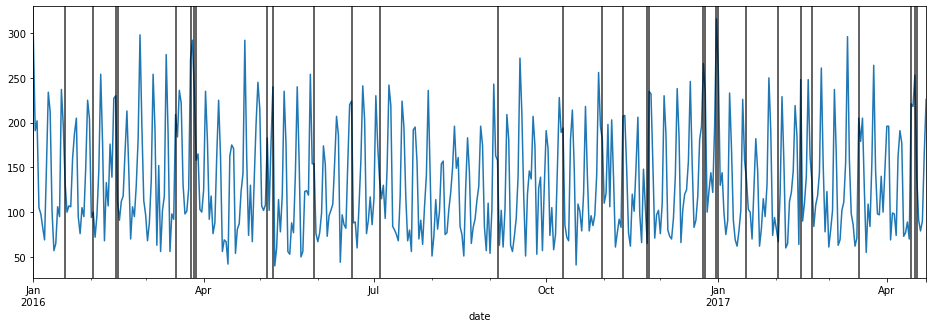
ax = df1['total'].plot(figsize=(16,5))

for day in df1.query('holiday==1').index:
    ax.axvline(x=day, color='k',alpha=.8);
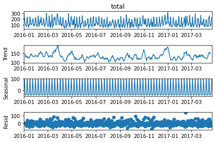
from statsmodels.tsa.seasonal import seasonal_decompose
result = seasonal_decompose(df1['total'])
result.plot();
result.seasonal.plot(figsize=(18,5))
<AxesSubplot:xlabel='date'>
len(df1)
478
train = df1.iloc[:436]
test = df1.iloc[436:]
from pmdarima import auto_arima
auto_arima(df1['total'], seasonal=True, m=7, trace=True).summary()
Performing stepwise search to minimize aic


C:\Users\ilvna\.conda\envs\tf-2.3\lib\site-packages\statsmodels\base\model.py:568: ConvergenceWarning: Maximum Likelihood optimization failed to converge. Check mle_retvals
  "Check mle_retvals", ConvergenceWarning)


 ARIMA(2,0,2)(1,0,1)[7] intercept   : AIC=inf, Time=1.72 sec
 ARIMA(0,0,0)(0,0,0)[7] intercept   : AIC=5269.484, Time=0.02 sec
 ARIMA(1,0,0)(1,0,0)[7] intercept   : AIC=4916.749, Time=0.46 sec
 ARIMA(0,0,1)(0,0,1)[7] intercept   : AIC=5049.644, Time=0.25 sec
 ARIMA(0,0,0)(0,0,0)[7]             : AIC=6126.084, Time=0.01 sec
 ARIMA(1,0,0)(0,0,0)[7] intercept   : AIC=5200.790, Time=0.06 sec
 ARIMA(1,0,0)(2,0,0)[7] intercept   : AIC=4845.442, Time=1.05 sec
 ARIMA(1,0,0)(2,0,1)[7] intercept   : AIC=inf, Time=nan sec


C:\Users\ilvna\.conda\envs\tf-2.3\lib\site-packages\statsmodels\base\model.py:568: ConvergenceWarning: Maximum Likelihood optimization failed to converge. Check mle_retvals
  "Check mle_retvals", ConvergenceWarning)


 ARIMA(1,0,0)(1,0,1)[7] intercept   : AIC=4805.859, Time=0.63 sec
 ARIMA(1,0,0)(0,0,1)[7] intercept   : AIC=5058.642, Time=0.37 sec


C:\Users\ilvna\.conda\envs\tf-2.3\lib\site-packages\statsmodels\base\model.py:568: ConvergenceWarning: Maximum Likelihood optimization failed to converge. Check mle_retvals
  "Check mle_retvals", ConvergenceWarning)


 ARIMA(1,0,0)(1,0,2)[7] intercept   : AIC=4948.132, Time=1.39 sec
 ARIMA(1,0,0)(0,0,2)[7] intercept   : AIC=4982.776, Time=0.64 sec


C:\Users\ilvna\.conda\envs\tf-2.3\lib\site-packages\statsmodels\base\model.py:568: ConvergenceWarning: Maximum Likelihood optimization failed to converge. Check mle_retvals
  "Check mle_retvals", ConvergenceWarning)


 ARIMA(1,0,0)(2,0,2)[7] intercept   : AIC=inf, Time=1.78 sec


C:\Users\ilvna\.conda\envs\tf-2.3\lib\site-packages\statsmodels\base\model.py:568: ConvergenceWarning: Maximum Likelihood optimization failed to converge. Check mle_retvals
  "Check mle_retvals", ConvergenceWarning)


 ARIMA(0,0,0)(1,0,1)[7] intercept   : AIC=4780.356, Time=0.66 sec
 ARIMA(0,0,0)(0,0,1)[7] intercept   : AIC=5093.130, Time=0.12 sec
 ARIMA(0,0,0)(1,0,0)[7] intercept   : AIC=4926.360, Time=0.31 sec
 ARIMA(0,0,0)(2,0,1)[7] intercept   : AIC=inf, Time=nan sec


C:\Users\ilvna\.conda\envs\tf-2.3\lib\site-packages\statsmodels\base\model.py:568: ConvergenceWarning: Maximum Likelihood optimization failed to converge. Check mle_retvals
  "Check mle_retvals", ConvergenceWarning)


 ARIMA(0,0,0)(1,0,2)[7] intercept   : AIC=4887.689, Time=1.07 sec
 ARIMA(0,0,0)(0,0,2)[7] intercept   : AIC=5010.582, Time=0.50 sec


C:\Users\ilvna\.conda\envs\tf-2.3\lib\site-packages\statsmodels\base\model.py:568: ConvergenceWarning: Maximum Likelihood optimization failed to converge. Check mle_retvals
  "Check mle_retvals", ConvergenceWarning)


 ARIMA(0,0,0)(2,0,0)[7] intercept   : AIC=4859.657, Time=1.26 sec
 ARIMA(0,0,0)(2,0,2)[7] intercept   : AIC=inf, Time=nan sec
 ARIMA(0,0,1)(1,0,1)[7] intercept   : AIC=inf, Time=0.80 sec


C:\Users\ilvna\.conda\envs\tf-2.3\lib\site-packages\statsmodels\base\model.py:568: ConvergenceWarning: Maximum Likelihood optimization failed to converge. Check mle_retvals
  "Check mle_retvals", ConvergenceWarning)


 ARIMA(1,0,1)(1,0,1)[7] intercept   : AIC=inf, Time=0.86 sec
 ARIMA(0,0,0)(1,0,1)[7]             : AIC=inf, Time=0.23 sec

Best model:  ARIMA(0,0,0)(1,0,1)[7] intercept
Total fit time: 17.200 seconds
| Dep. Variable: | y | No. Observations: | 478 |
|---|---|---|---|
| Model: | SARIMAX(1, 0, [1], 7) | Log Likelihood | -2386.178 |
| Date: | Thu, 15 Oct 2020 | AIC | 4780.356 |
| Time: | 19:17:46 | BIC | 4797.035 |
| Sample: | 0 | HQIC | 4786.913 |
| - 478 | |||
| Covariance Type: | opg |
| coef | std err | z | P>|z| | [0.025 | 0.975] | |
|---|---|---|---|---|---|---|
| intercept | 5.6944 | 1.886 | 3.020 | 0.003 | 1.998 | 9.391 |
| ar.S.L7 | 0.9571 | 0.014 | 67.726 | 0.000 | 0.929 | 0.985 |
| ma.S.L7 | -0.7553 | 0.050 | -15.001 | 0.000 | -0.854 | -0.657 |
| sigma2 | 1244.1294 | 74.922 | 16.606 | 0.000 | 1097.285 | 1390.973 |
| Ljung-Box (Q): | 74.35 | Jarque-Bera (JB): | 61.36 |
|---|---|---|---|
| Prob(Q): | 0.00 | Prob(JB): | 0.00 |
| Heteroskedasticity (H): | 0.85 | Skew: | 0.75 |
| Prob(H) (two-sided): | 0.30 | Kurtosis: | 3.92 |
Warnings:
[1] Covariance matrix calculated using the outer product of gradients (complex-step).
from statsmodels.tsa.statespace.sarimax import SARIMAX
# ValueError: non-invertible starting MA parameters found

model = SARIMAX(train['total'], order=(1,0,0), seasonal_order=(2,0,0,7),
               enforce_invertibility=False)
model_c = SARIMAX(train['total'], order=(0,0,0), seasonal_order=(1,0,1,7),
               enforce_invertibility=False)
results = model.fit()
results_c = model_c.fit()
results.summary()
| Dep. Variable: | total | No. Observations: | 436 |
|---|---|---|---|
| Model: | SARIMAX(1, 0, 0)x(2, 0, 0, 7) | Log Likelihood | -2224.701 |
| Date: | Thu, 15 Oct 2020 | AIC | 4457.403 |
| Time: | 19:17:47 | BIC | 4473.713 |
| Sample: | 01-01-2016 | HQIC | 4463.840 |
| - 03-11-2017 | |||
| Covariance Type: | opg |
| coef | std err | z | P>|z| | [0.025 | 0.975] | |
|---|---|---|---|---|---|---|
| ar.L1 | 0.2212 | 0.047 | 4.711 | 0.000 | 0.129 | 0.313 |
| ar.S.L7 | 0.5063 | 0.036 | 14.187 | 0.000 | 0.436 | 0.576 |
| ar.S.L14 | 0.4574 | 0.037 | 12.379 | 0.000 | 0.385 | 0.530 |
| sigma2 | 1520.2899 | 82.277 | 18.478 | 0.000 | 1359.029 | 1681.550 |
| Ljung-Box (Q): | 83.96 | Jarque-Bera (JB): | 29.23 |
|---|---|---|---|
| Prob(Q): | 0.00 | Prob(JB): | 0.00 |
| Heteroskedasticity (H): | 0.86 | Skew: | 0.34 |
| Prob(H) (two-sided): | 0.37 | Kurtosis: | 4.07 |
Warnings:
[1] Covariance matrix calculated using the outer product of gradients (complex-step).
results_c.summary()
| Dep. Variable: | total | No. Observations: | 436 |
|---|---|---|---|
| Model: | SARIMAX(1, 0, [1], 7) | Log Likelihood | -2165.369 |
| Date: | Thu, 15 Oct 2020 | AIC | 4336.738 |
| Time: | 19:17:47 | BIC | 4348.970 |
| Sample: | 01-01-2016 | HQIC | 4341.565 |
| - 03-11-2017 | |||
| Covariance Type: | opg |
| coef | std err | z | P>|z| | [0.025 | 0.975] | |
|---|---|---|---|---|---|---|
| ar.S.L7 | 0.9999 | 9.57e-05 | 1.04e+04 | 0.000 | 1.000 | 1.000 |
| ma.S.L7 | -0.9384 | 0.024 | -39.206 | 0.000 | -0.985 | -0.891 |
| sigma2 | 1111.7950 | 58.740 | 18.927 | 0.000 | 996.667 | 1226.923 |
| Ljung-Box (Q): | 67.58 | Jarque-Bera (JB): | 83.57 |
|---|---|---|---|
| Prob(Q): | 0.00 | Prob(JB): | 0.00 |
| Heteroskedasticity (H): | 0.96 | Skew: | 0.72 |
| Prob(H) (two-sided): | 0.81 | Kurtosis: | 4.59 |
Warnings:
[1] Covariance matrix calculated using the outer product of gradients (complex-step).
start = len(train)
end = len(train) + len(test) - 1
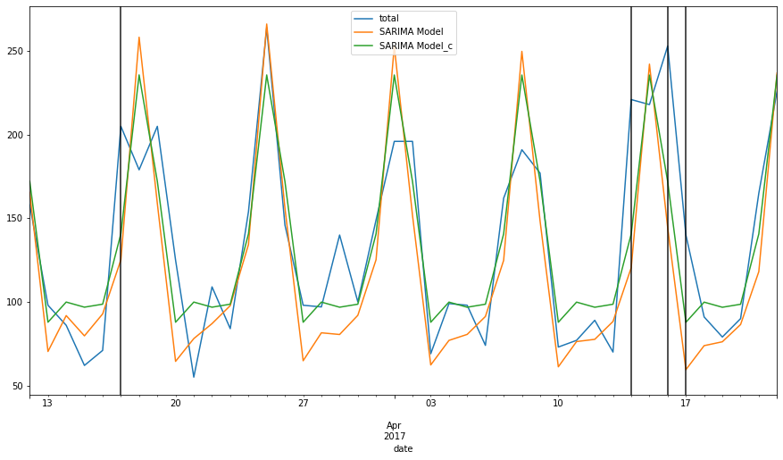
predictions = results.predict(start, end).rename('SARIMA Model')
predictions_c = results_c.predict(start,end).rename('SARIMA Model_c')
ax = test['total'].plot(figsize=(15,8), legend=True)
predictions.plot(legend=True)
predictions_c.plot(legend=True)

for day in test.query('holiday==1').index:
    ax.axvline(x=day, color='k',alpha=.9);
from statsmodels.tools.eval_measures import rmse
print(rmse(test['total'], predictions))
print(rmse(test['total'], predictions_c))
print(test['total'].mean())
print(predictions.mean())
print(predictions_c.mean())
41.26315495065604
31.912579096986363
134.26190476190476
120.72598706500457
133.08493968389868
# df1[['holiday']]
auto_arima(df1['total'], exogenous=df1[['holiday']],seasonal=True,m=7, trace=True).summary()
Performing stepwise search to minimize aic


C:\Users\ilvna\.conda\envs\tf-2.3\lib\site-packages\statsmodels\base\model.py:568: ConvergenceWarning: Maximum Likelihood optimization failed to converge. Check mle_retvals
  "Check mle_retvals", ConvergenceWarning)


 ARIMA(2,0,2)(1,0,1)[7] intercept   : AIC=inf, Time=1.47 sec
 ARIMA(0,0,0)(0,0,0)[7] intercept   : AIC=5235.582, Time=0.07 sec


C:\Users\ilvna\.conda\envs\tf-2.3\lib\site-packages\statsmodels\base\model.py:568: ConvergenceWarning: Maximum Likelihood optimization failed to converge. Check mle_retvals
  "Check mle_retvals", ConvergenceWarning)


 ARIMA(1,0,0)(1,0,0)[7] intercept   : AIC=4804.111, Time=0.70 sec
 ARIMA(0,0,1)(0,0,1)[7] intercept   : AIC=4969.638, Time=0.51 sec
 ARIMA(0,0,0)(0,0,0)[7]             : AIC=6068.575, Time=0.07 sec
 ARIMA(1,0,0)(0,0,0)[7] intercept   : AIC=5171.193, Time=0.20 sec


C:\Users\ilvna\.conda\envs\tf-2.3\lib\site-packages\statsmodels\base\model.py:568: ConvergenceWarning: Maximum Likelihood optimization failed to converge. Check mle_retvals
  "Check mle_retvals", ConvergenceWarning)


 ARIMA(1,0,0)(2,0,0)[7] intercept   : AIC=inf, Time=1.39 sec


C:\Users\ilvna\.conda\envs\tf-2.3\lib\site-packages\statsmodels\base\model.py:568: ConvergenceWarning: Maximum Likelihood optimization failed to converge. Check mle_retvals
  "Check mle_retvals", ConvergenceWarning)


 ARIMA(1,0,0)(1,0,1)[7] intercept   : AIC=4728.053, Time=0.66 sec
 ARIMA(1,0,0)(0,0,1)[7] intercept   : AIC=4990.373, Time=0.48 sec


C:\Users\ilvna\.conda\envs\tf-2.3\lib\site-packages\statsmodels\base\model.py:568: ConvergenceWarning: Maximum Likelihood optimization failed to converge. Check mle_retvals
  "Check mle_retvals", ConvergenceWarning)


 ARIMA(1,0,0)(2,0,1)[7] intercept   : AIC=inf, Time=1.41 sec


C:\Users\ilvna\.conda\envs\tf-2.3\lib\site-packages\statsmodels\base\model.py:568: ConvergenceWarning: Maximum Likelihood optimization failed to converge. Check mle_retvals
  "Check mle_retvals", ConvergenceWarning)


 ARIMA(1,0,0)(1,0,2)[7] intercept   : AIC=4812.844, Time=1.24 sec
 ARIMA(1,0,0)(0,0,2)[7] intercept   : AIC=4887.554, Time=1.04 sec


C:\Users\ilvna\.conda\envs\tf-2.3\lib\site-packages\statsmodels\base\model.py:568: ConvergenceWarning: Maximum Likelihood optimization failed to converge. Check mle_retvals
  "Check mle_retvals", ConvergenceWarning)


 ARIMA(1,0,0)(2,0,2)[7] intercept   : AIC=inf, Time=1.65 sec


C:\Users\ilvna\.conda\envs\tf-2.3\lib\site-packages\statsmodels\base\model.py:568: ConvergenceWarning: Maximum Likelihood optimization failed to converge. Check mle_retvals
  "Check mle_retvals", ConvergenceWarning)


 ARIMA(0,0,0)(1,0,1)[7] intercept   : AIC=4829.768, Time=0.62 sec


C:\Users\ilvna\.conda\envs\tf-2.3\lib\site-packages\statsmodels\base\model.py:568: ConvergenceWarning: Maximum Likelihood optimization failed to converge. Check mle_retvals
  "Check mle_retvals", ConvergenceWarning)


 ARIMA(2,0,0)(1,0,1)[7] intercept   : AIC=5148.817, Time=0.97 sec


C:\Users\ilvna\.conda\envs\tf-2.3\lib\site-packages\statsmodels\base\model.py:568: ConvergenceWarning: Maximum Likelihood optimization failed to converge. Check mle_retvals
  "Check mle_retvals", ConvergenceWarning)


 ARIMA(1,0,1)(1,0,1)[7] intercept   : AIC=inf, Time=0.90 sec


C:\Users\ilvna\.conda\envs\tf-2.3\lib\site-packages\statsmodels\base\model.py:568: ConvergenceWarning: Maximum Likelihood optimization failed to converge. Check mle_retvals
  "Check mle_retvals", ConvergenceWarning)


 ARIMA(0,0,1)(1,0,1)[7] intercept   : AIC=4782.008, Time=0.79 sec


C:\Users\ilvna\.conda\envs\tf-2.3\lib\site-packages\statsmodels\base\model.py:568: ConvergenceWarning: Maximum Likelihood optimization failed to converge. Check mle_retvals
  "Check mle_retvals", ConvergenceWarning)


 ARIMA(2,0,1)(1,0,1)[7] intercept   : AIC=inf, Time=1.02 sec
 ARIMA(1,0,0)(1,0,1)[7]             : AIC=inf, Time=0.57 sec

Best model:  ARIMA(1,0,0)(1,0,1)[7] intercept
Total fit time: 15.776 seconds


C:\Users\ilvna\.conda\envs\tf-2.3\lib\site-packages\statsmodels\base\model.py:568: ConvergenceWarning: Maximum Likelihood optimization failed to converge. Check mle_retvals
  "Check mle_retvals", ConvergenceWarning)
| Dep. Variable: | y | No. Observations: | 478 |
|---|---|---|---|
| Model: | SARIMAX(1, 0, 0)x(1, 0, [1], 7) | Log Likelihood | -2358.026 |
| Date: | Thu, 15 Oct 2020 | AIC | 4728.053 |
| Time: | 19:18:35 | BIC | 4753.070 |
| Sample: | 01-01-2016 | HQIC | 4737.888 |
| - 04-22-2017 | |||
| Covariance Type: | opg |
| coef | std err | z | P>|z| | [0.025 | 0.975] | |
|---|---|---|---|---|---|---|
| intercept | 19.0587 | 2.907 | 6.557 | 0.000 | 13.362 | 24.755 |
| holiday | 52.1120 | 3.981 | 13.089 | 0.000 | 44.309 | 59.915 |
| ar.L1 | 0.1580 | 0.042 | 3.768 | 0.000 | 0.076 | 0.240 |
| ar.S.L7 | 0.8269 | 0.024 | 34.166 | 0.000 | 0.779 | 0.874 |
| ma.S.L7 | -0.3437 | 0.056 | -6.180 | 0.000 | -0.453 | -0.235 |
| sigma2 | 971.3466 | 61.369 | 15.828 | 0.000 | 851.066 | 1091.628 |
| Ljung-Box (Q): | 109.04 | Jarque-Bera (JB): | 7.00 |
|---|---|---|---|
| Prob(Q): | 0.00 | Prob(JB): | 0.03 |
| Heteroskedasticity (H): | 0.91 | Skew: | 0.29 |
| Prob(H) (two-sided): | 0.55 | Kurtosis: | 3.13 |
Warnings:
[1] Covariance matrix calculated using the outer product of gradients (complex-step).
Train out SARIMAX
model = SARIMAX(train['total'],exog=train[['holiday']],order=(1,0,1),
               seasonal_order=(1,0,1,7), enforce_invertibility=False)
model_c = SARIMAX(train['total'], exog=train[['holiday']], order=(1,0,0),
                 seasonal_order=(1,0,1,7), enforce_invertibility=False)
result = model.fit()
result_c = model_c.fit()
C:\Users\ilvna\.conda\envs\tf-2.3\lib\site-packages\statsmodels\base\model.py:568: ConvergenceWarning: Maximum Likelihood optimization failed to converge. Check mle_retvals
  "Check mle_retvals", ConvergenceWarning)
result.summary()
| Dep. Variable: | total | No. Observations: | 436 |
|---|---|---|---|
| Model: | SARIMAX(1, 0, 1)x(1, 0, 1, 7) | Log Likelihood | -2175.956 |
| Date: | Thu, 15 Oct 2020 | AIC | 4363.911 |
| Time: | 19:19:25 | BIC | 4388.377 |
| Sample: | 01-01-2016 | HQIC | 4373.567 |
| - 03-11-2017 | |||
| Covariance Type: | opg |
| coef | std err | z | P>|z| | [0.025 | 0.975] | |
|---|---|---|---|---|---|---|
| holiday | 119.2207 | 3.207 | 37.177 | 0.000 | 112.935 | 125.506 |
| ar.L1 | 0.9997 | 0.000 | 2763.806 | 0.000 | 0.999 | 1.000 |
| ma.L1 | -1.7406 | 0.089 | -19.564 | 0.000 | -1.915 | -1.566 |
| ar.S.L7 | 0.9997 | 0.001 | 1799.530 | 0.000 | 0.999 | 1.001 |
| ma.S.L7 | -1.0307 | 0.025 | -41.893 | 0.000 | -1.079 | -0.982 |
| sigma2 | 289.5149 | 20.075 | 14.422 | 0.000 | 250.169 | 328.861 |
| Ljung-Box (Q): | 77.56 | Jarque-Bera (JB): | 99.68 |
|---|---|---|---|
| Prob(Q): | 0.00 | Prob(JB): | 0.00 |
| Heteroskedasticity (H): | 1.05 | Skew: | -0.54 |
| Prob(H) (two-sided): | 0.77 | Kurtosis: | 5.08 |
Warnings:
[1] Covariance matrix calculated using the outer product of gradients (complex-step).
result_c.summary()
| Dep. Variable: | total | No. Observations: | 436 |
|---|---|---|---|
| Model: | SARIMAX(1, 0, 0)x(1, 0, [1], 7) | Log Likelihood | -2089.208 |
| Date: | Thu, 15 Oct 2020 | AIC | 4188.417 |
| Time: | 19:19:25 | BIC | 4208.805 |
| Sample: | 01-01-2016 | HQIC | 4196.463 |
| - 03-11-2017 | |||
| Covariance Type: | opg |
| coef | std err | z | P>|z| | [0.025 | 0.975] | |
|---|---|---|---|---|---|---|
| holiday | 68.9355 | 3.773 | 18.271 | 0.000 | 61.541 | 76.330 |
| ar.L1 | 0.2101 | 0.044 | 4.763 | 0.000 | 0.124 | 0.297 |
| ar.S.L7 | 1.0000 | 5.78e-05 | 1.73e+04 | 0.000 | 1.000 | 1.000 |
| ma.S.L7 | -0.9581 | 0.022 | -43.532 | 0.000 | -1.001 | -0.915 |
| sigma2 | 779.3163 | 44.867 | 17.369 | 0.000 | 691.378 | 867.254 |
| Ljung-Box (Q): | 36.17 | Jarque-Bera (JB): | 20.47 |
|---|---|---|---|
| Prob(Q): | 0.64 | Prob(JB): | 0.00 |
| Heteroskedasticity (H): | 0.98 | Skew: | 0.22 |
| Prob(H) (two-sided): | 0.88 | Kurtosis: | 3.96 |
Warnings:
[1] Covariance matrix calculated using the outer product of gradients (complex-step).
start = len(train)
end = len(train) + len(test) - 1
predictions = result.predict(start, end, exog=test[['holiday']]).rename('SARIMAX with Exog')
predictions_c = result_c.predict(start, end, exog=test[['holiday']]).rename('SARIMAX with Exog c')
ax = test['total'].plot(figsize=(12,8), legend=True)
predictions.plot(legend=True)
predictions_c.plot(legend=True)


for day in test.query('holiday==1').index:
    ax.axvline(x=day, color='k',alpha=.9);
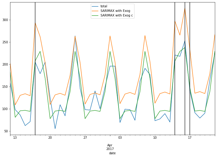
print(rmse(test['total'], predictions))
print(rmse(test['total'], predictions_c))
print(test['total'].mean())
print(predictions.mean())
print(predictions_c.mean())
49.92655128660368
22.92975136294346
134.26190476190476
176.6705414607891
135.4431981814327
FORECAST
model = SARIMAX(df1['total'],exog=df1[['holiday']], order=(1,0,1),
               seasonal_order=(1,0,1,7), enforce_invertibility=False)
model_c = SARIMAX(df1['total'], exog=df1[['holiday']], order=(1,0,0),
                 seasonal_order=(1,0,1,7), enforce_invertibility=False)
results = model.fit()
results_c = model_c.fit()
exog_forecast = df[478:][['holiday']]
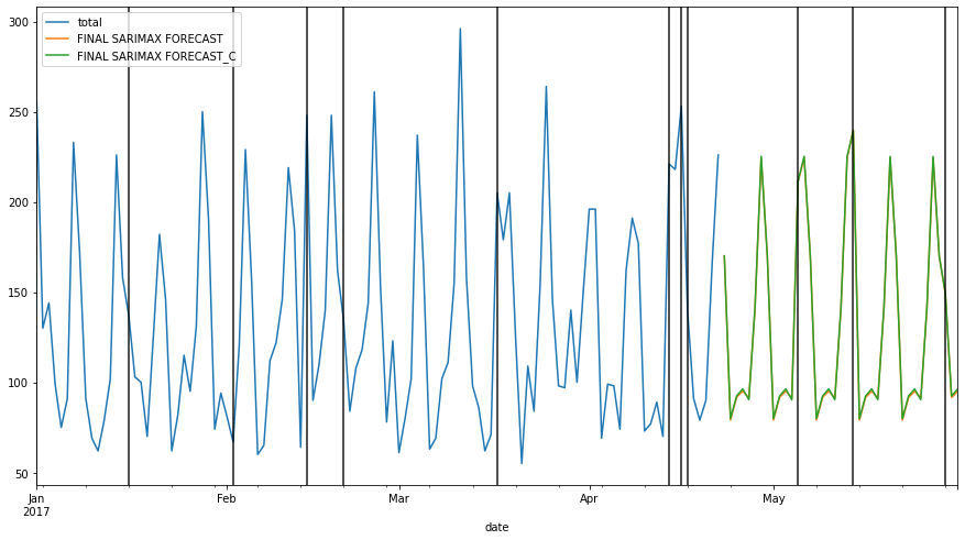
fcast = results.predict(len(df1),len(df1)+38, exog = exog_forecast).rename('FINAL SARIMAX FORECAST')
fcast_c = results_c.predict(len(df1), len(df1)+38, exog = exog_forecast).rename('FINAL SARIMAX FORECAST_C')
ax = df1['total'].loc['2017-01-01':].plot(figsize=(15,8), legend=True)
fcast.plot(legend=True)
fcast_c.plot(legend=True)

for day in df.query('holiday==1').index:
    ax.axvline(x=day, color='k',alpha=.9);
from statsmodels.tools.eval_measures import rmse
rmse(fcast, fcast_c)
0.8548258765517648