Time series - Alcohol Sales
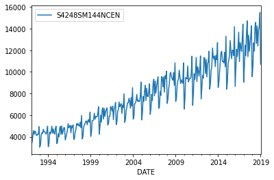
Alcohol Sales
import pandas as pd
import numpy as np

import matplotlib.pyplot as plt
import warnings
warnings.filterwarnings('ignore')
df = pd.read_csv('./Data/Alcohol_Sales.csv', index_col='DATE', parse_dates=True)
df.index.freq = 'MS'
df.info()
<class 'pandas.core.frame.DataFrame'>
DatetimeIndex: 325 entries, 1992-01-01 to 2019-01-01
Freq: MS
Data columns (total 1 columns):
 #   Column          Non-Null Count  Dtype
---  ------          --------------  -----
 0   S4248SM144NCEN  325 non-null    int64
dtypes: int64(1)
memory usage: 5.1 KB
df.plot()
plt.show()
General Forecasting Model
from statsmodels.tsa.holtwinters import ExponentialSmoothing
from sklearn.metrics import mean_absolute_error, mean_squared_error
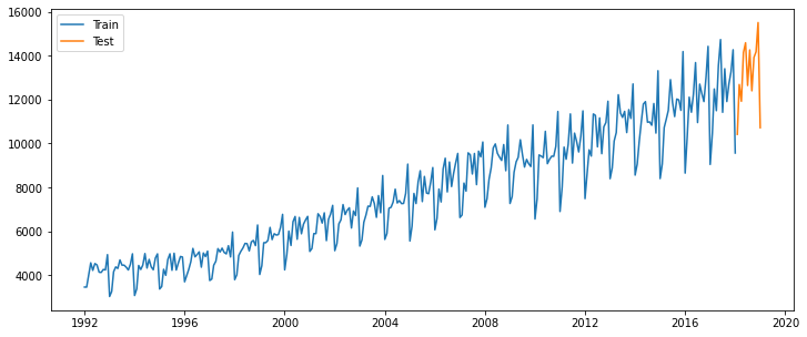
train_data = df.iloc[:-12]
test_data = df.iloc[-12:]
print(df.shape)
print(train_data.shape)
print(test_data.shape)
(325, 1)
(313, 1)
(12, 1)
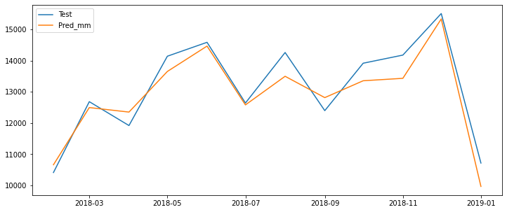
fitted_model_mm = ExponentialSmoothing(train_data, trend='mul', seasonal='mul',seasonal_periods=12).fit()
fitted_model_aa = ExponentialSmoothing(train_data, trend='add', seasonal='add',seasonal_periods=12).fit()
c:\users\ilvna\.conda\envs\tf\lib\site-packages\statsmodels\tsa\holtwinters\model.py:922: ConvergenceWarning: Optimization failed to converge. Check mle_retvals.
  ConvergenceWarning,
test_predictions_mm = fitted_model.forecast(12)
test_predictions_aa = fitted_model.forecast(12)
plt.figure(figsize=(12,5))
plt.plot(train_data, label='Train')
plt.plot(test_data, label='Test')
plt.legend()
plt.show()
plt.figure(figsize=(12,5))
plt.plot(test_data, label='Test')
plt.plot(test_predictions_mm, label='Pred_mm')
plt.legend()
plt.show()
mae = mean_absolute_error(test_data, test_predictions)
mse = mean_squared_error(test_data ,test_predictions)
rmse = np.sqrt(mse)
print('mae :', mae)
print('mse :', mse)
print('rmse :', rmse)
mae : 411.9015865536535
mse : 229275.45568794024
rmse : 478.82716682320796
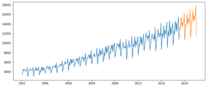
final_model = ExponentialSmoothing(df, trend='mul', seasonal='mul', seasonal_periods=12).fit()
c:\users\ilvna\.conda\envs\tf\lib\site-packages\statsmodels\tsa\holtwinters\model.py:922: ConvergenceWarning: Optimization failed to converge. Check mle_retvals.
  ConvergenceWarning,
forecast_prediction = final_model.forecast(36)
plt.figure(figsize=(12,5))
plt.plot(df)
plt.plot(forecast_prediction)
plt.show()
ARIMA
from statsmodels.tsa.stattools import adfuller
from pmdarima import auto_arima

from statsmodels.tsa.arima_model import ARMA, ARIMA, ARMAResults, ARIMAResults
from statsmodels.tsa.statespace.sarimax import SARIMAX, SARIMAXResults
from statsmodels.graphics.tsaplots import plot_acf, plot_pacf
from statsmodels.tsa.statespace.tools import diff
from statsmodels.tsa.seasonal import seasonal_decompose
from statsmodels.graphics.tsaplots import plot_acf, plot_pacf
from statsmodels.tools.eval_measures import rmse
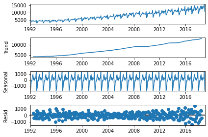
result = seasonal_decompose(df, model='add')
result.plot()
plt.show()
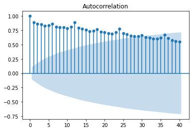
plot_acf(df, lags=40)
plt.show()
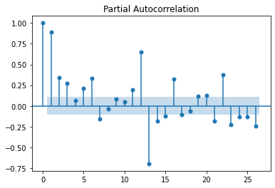
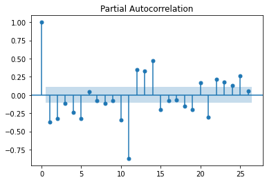
plot_pacf(df)
plt.show()
df_log = np.log(df)
df_log_diff = diff(df_log)
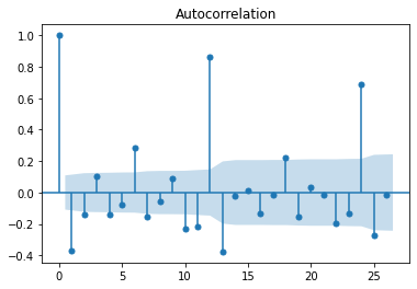
plot_acf(df_log_diff)
plot_pacf(df_log_diff)
plt.show()
print('p-value is : {}'.format(adfuller(df)[1]))
p-value is : 0.9987196267088919
isn’t stationary
df_diff = diff(df, k_diff=1)
print('p-value is : {}'.format(adfuller(df_diff)[1]))
p-value is : 0.0003408284921168574
is stationary
auto_arima
stepwise_fit = auto_arima(df, seasonal=True, trace=True, m=12)
Performing stepwise search to minimize aic
 ARIMA(2,1,2)(1,1,1)[12]             : AIC=4514.024, Time=1.35 sec
 ARIMA(0,1,0)(0,1,0)[12]             : AIC=4868.181, Time=0.01 sec
 ARIMA(1,1,0)(1,1,0)[12]             : AIC=4731.674, Time=0.08 sec
 ARIMA(0,1,1)(0,1,1)[12]             : AIC=4629.449, Time=0.66 sec
 ARIMA(2,1,2)(0,1,1)[12]             : AIC=4527.109, Time=0.79 sec
 ARIMA(2,1,2)(1,1,0)[12]             : AIC=4539.016, Time=0.39 sec
 ARIMA(2,1,2)(2,1,1)[12]             : AIC=4499.168, Time=4.80 sec
 ARIMA(2,1,2)(2,1,0)[12]             : AIC=4523.762, Time=1.18 sec
 ARIMA(2,1,2)(2,1,2)[12]             : AIC=inf, Time=7.26 sec
 ARIMA(2,1,2)(1,1,2)[12]             : AIC=4508.118, Time=4.54 sec
 ARIMA(1,1,2)(2,1,1)[12]             : AIC=4526.711, Time=5.72 sec
 ARIMA(2,1,1)(2,1,1)[12]             : AIC=4504.012, Time=3.65 sec
 ARIMA(3,1,2)(2,1,1)[12]             : AIC=4491.408, Time=5.70 sec
 ARIMA(3,1,2)(1,1,1)[12]             : AIC=4506.197, Time=2.39 sec
 ARIMA(3,1,2)(2,1,0)[12]             : AIC=4514.299, Time=4.16 sec
 ARIMA(3,1,2)(2,1,2)[12]             : AIC=4444.011, Time=7.65 sec
 ARIMA(3,1,2)(1,1,2)[12]             : AIC=4499.385, Time=6.75 sec
 ARIMA(3,1,1)(2,1,2)[12]             : AIC=inf, Time=6.98 sec
 ARIMA(4,1,2)(2,1,2)[12]             : AIC=4460.069, Time=9.64 sec
 ARIMA(3,1,3)(2,1,2)[12]             : AIC=4448.232, Time=9.26 sec
 ARIMA(2,1,1)(2,1,2)[12]             : AIC=inf, Time=6.27 sec
 ARIMA(2,1,3)(2,1,2)[12]             : AIC=4449.248, Time=8.97 sec
 ARIMA(4,1,1)(2,1,2)[12]             : AIC=inf, Time=8.59 sec
 ARIMA(4,1,3)(2,1,2)[12]             : AIC=4460.041, Time=10.26 sec
 ARIMA(3,1,2)(2,1,2)[12] intercept   : AIC=4462.884, Time=8.87 sec

Best model:  ARIMA(3,1,2)(2,1,2)[12]
Total fit time: 125.962 seconds
stepwise_fit.summary()
| Dep. Variable: | y | No. Observations: | 325 |
|---|---|---|---|
| Model: | SARIMAX(3, 1, 2)x(2, 1, 2, 12) | Log Likelihood | -2212.006 |
| Date: | Fri, 09 Apr 2021 | AIC | 4444.011 |
| Time: | 11:46:26 | BIC | 4481.441 |
| Sample: | 0 | HQIC | 4458.971 |
| - 325 | |||
| Covariance Type: | opg |
| coef | std err | z | P>|z| | [0.025 | 0.975] | |
|---|---|---|---|---|---|---|
| ar.L1 | -0.0899 | 0.215 | -0.418 | 0.676 | -0.512 | 0.332 |
| ar.L2 | 0.0985 | 0.087 | 1.128 | 0.259 | -0.073 | 0.270 |
| ar.L3 | 0.3208 | 0.069 | 4.639 | 0.000 | 0.185 | 0.456 |
| ma.L1 | -0.7431 | 0.223 | -3.335 | 0.001 | -1.180 | -0.306 |
| ma.L2 | -0.1539 | 0.182 | -0.845 | 0.398 | -0.511 | 0.203 |
| ar.S.L12 | 0.8702 | 0.068 | 12.850 | 0.000 | 0.737 | 1.003 |
| ar.S.L24 | -0.8249 | 0.059 | -13.973 | 0.000 | -0.941 | -0.709 |
| ma.S.L12 | -1.1483 | 0.100 | -11.534 | 0.000 | -1.343 | -0.953 |
| ma.S.L24 | 0.6663 | 0.096 | 6.959 | 0.000 | 0.479 | 0.854 |
| sigma2 | 8.337e+04 | 6834.224 | 12.199 | 0.000 | 7e+04 | 9.68e+04 |
| Ljung-Box (L1) (Q): | 0.18 | Jarque-Bera (JB): | 10.24 |
|---|---|---|---|
| Prob(Q): | 0.67 | Prob(JB): | 0.01 |
| Heteroskedasticity (H): | 4.23 | Skew: | -0.11 |
| Prob(H) (two-sided): | 0.00 | Kurtosis: | 3.86 |
Warnings:
[1] Covariance matrix calculated using the outer product of gradients (complex-step).
model = SARIMAX(train_data, order=(3,1,2), seasonal_order=(2,1,2,12))
results = model.fit()
c:\users\ilvna\.conda\envs\tf\lib\site-packages\statsmodels\base\model.py:568: ConvergenceWarning: Maximum Likelihood optimization failed to converge. Check mle_retvals
  ConvergenceWarning)
results.summary()
| Dep. Variable: | S4248SM144NCEN | No. Observations: | 313 |
|---|---|---|---|
| Model: | SARIMAX(3, 1, 2)x(2, 1, 2, 12) | Log Likelihood | -2130.091 |
| Date: | Fri, 09 Apr 2021 | AIC | 4280.183 |
| Time: | 11:47:17 | BIC | 4317.221 |
| Sample: | 01-01-1992 | HQIC | 4295.005 |
| - 01-01-2018 | |||
| Covariance Type: | opg |
| coef | std err | z | P>|z| | [0.025 | 0.975] | |
|---|---|---|---|---|---|---|
| ar.L1 | -0.2578 | 0.223 | -1.158 | 0.247 | -0.694 | 0.178 |
| ar.L2 | 0.0882 | 0.104 | 0.845 | 0.398 | -0.116 | 0.293 |
| ar.L3 | 0.3605 | 0.085 | 4.235 | 0.000 | 0.194 | 0.527 |
| ma.L1 | -0.6401 | 0.225 | -2.844 | 0.004 | -1.081 | -0.199 |
| ma.L2 | -0.2576 | 0.188 | -1.373 | 0.170 | -0.625 | 0.110 |
| ar.S.L12 | 0.8397 | 0.124 | 6.754 | 0.000 | 0.596 | 1.083 |
| ar.S.L24 | -0.7472 | 0.087 | -8.554 | 0.000 | -0.918 | -0.576 |
| ma.S.L12 | -1.1464 | 0.158 | -7.235 | 0.000 | -1.457 | -0.836 |
| ma.S.L24 | 0.6295 | 0.149 | 4.230 | 0.000 | 0.338 | 0.921 |
| sigma2 | 1.02e+05 | 1.01e+04 | 10.119 | 0.000 | 8.22e+04 | 1.22e+05 |
| Ljung-Box (L1) (Q): | 0.17 | Jarque-Bera (JB): | 9.97 |
|---|---|---|---|
| Prob(Q): | 0.68 | Prob(JB): | 0.01 |
| Heteroskedasticity (H): | 4.70 | Skew: | -0.12 |
| Prob(H) (two-sided): | 0.00 | Kurtosis: | 3.86 |
Warnings:
[1] Covariance matrix calculated using the outer product of gradients (complex-step).
start = len(train_data)
end = len(train_data) + len(test_data) - 1
pred = results.predict(start, end, typ='level')
plt.plot(test_data)
plt.plot(pred)
plt.show()
error = rmse(test_data, pred)
error
array([2854.34960749, 1718.78826431, 1867.1512623 , 1812.19483997,
       2065.05758019, 1687.09691322, 1590.03025873, 1711.93822433,
       1559.00525313, 1517.72740288, 2247.46882941, 3260.6541987 ])
model = SARIMAX(df, order=(3,1,2), seasonal_order=(2,1,2,12))
results = model.fit()
c:\users\ilvna\.conda\envs\tf\lib\site-packages\statsmodels\base\model.py:568: ConvergenceWarning: Maximum Likelihood optimization failed to converge. Check mle_retvals
  ConvergenceWarning)
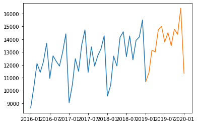
forecast = results.predict(len(df)-1, len(df)+11, typ='levels')
plt.plot(df['2016-01-01':])
plt.plot(forecast)
plt.show()
LSTM
from tensorflow.keras.preprocessing.sequence import TimeseriesGenerator
from sklearn.preprocessing import MinMaxScaler
from tensorflow.keras.models import Model
from tensorflow.keras.layers import Dense, LSTM, Input
nobs = 12
train = df.iloc[:-nobs]
test = df.iloc[-nobs:]
scaler = MinMaxScaler()
scaler.fit(train)
MinMaxScaler()
scaled_train = scaler.transform(train)
scaled_test = scaler.transform(test)
n_input = 12
n_features = 1

gen = TimeseriesGenerator(scaled_train, scaled_train, length=n_input, batch_size=1)
print(len(scaled_train))
print(len(scaled_test))
print(len(gen))
313
12
301
X, y = gen[0]
X, y
(array([[[0.03658432],
         [0.03649885],
         [0.08299855],
         [0.13103684],
         [0.1017181 ],
         [0.12804513],
         [0.12266006],
         [0.09453799],
         [0.09359774],
         [0.10496624],
         [0.10334217],
         [0.16283443]]]),
 array([[0.]]))
inputs = Input(shape=(n_input, n_features))
x = LSTM(150, activation='relu')(inputs)
x = Dense(1)(x)
WARNING:tensorflow:Layer lstm will not use cuDNN kernel since it doesn't meet the cuDNN kernel criteria. It will use generic GPU kernel as fallback when running on GPU
model = Model(inputs, x)
model.summary()
Model: "functional_1"
_________________________________________________________________
Layer (type)                 Output Shape              Param #
=================================================================
input_1 (InputLayer)         [(None, 12, 1)]           0
_________________________________________________________________
lstm (LSTM)                  (None, 150)               91200
_________________________________________________________________
dense (Dense)                (None, 1)                 151
=================================================================
Total params: 91,351
Trainable params: 91,351
Non-trainable params: 0
_________________________________________________________________
model.compile(optimizer='adam', loss='mse')
history = model.fit_generator(gen, epochs = 25)
Epoch 1/25
301/301 [==============================] - 5s 16ms/step - loss: 0.0096
Epoch 2/25
301/301 [==============================] - 5s 16ms/step - loss: 0.0094
Epoch 3/25
301/301 [==============================] - 5s 16ms/step - loss: 0.0087
Epoch 4/25
301/301 [==============================] - 5s 16ms/step - loss: 0.0066
Epoch 5/25
301/301 [==============================] - 5s 16ms/step - loss: 0.0054
Epoch 6/25
301/301 [==============================] - 5s 16ms/step - loss: 0.0039
Epoch 7/25
301/301 [==============================] - 5s 16ms/step - loss: 0.0035
Epoch 8/25
301/301 [==============================] - 5s 16ms/step - loss: 0.0031: 0s
Epoch 9/25
301/301 [==============================] - 5s 16ms/step - loss: 0.0025
Epoch 10/25
301/301 [==============================] - 5s 16ms/step - loss: 0.0021
Epoch 11/25
301/301 [==============================] - 5s 16ms/step - loss: 0.0022
Epoch 12/25
301/301 [==============================] - 5s 17ms/step - loss: 0.0023
Epoch 13/25
301/301 [==============================] - 5s 17ms/step - loss: 0.0024
Epoch 14/25
301/301 [==============================] - 5s 17ms/step - loss: 0.0021
Epoch 15/25
301/301 [==============================] - 5s 17ms/step - loss: 0.0017
Epoch 16/25
301/301 [==============================] - 5s 17ms/step - loss: 0.0016
Epoch 17/25
301/301 [==============================] - 5s 17ms/step - loss: 0.0020
Epoch 18/25
301/301 [==============================] - 5s 17ms/step - loss: 0.0018
Epoch 19/25
301/301 [==============================] - 5s 17ms/step - loss: 0.0017
Epoch 20/25
301/301 [==============================] - 5s 17ms/step - loss: 0.0015
Epoch 21/25
301/301 [==============================] - 5s 17ms/step - loss: 0.0017
Epoch 22/25
301/301 [==============================] - 5s 17ms/step - loss: 0.0018
Epoch 23/25
301/301 [==============================] - 5s 17ms/step - loss: 0.0017
Epoch 24/25
301/301 [==============================] - 5s 17ms/step - loss: 0.0019
Epoch 25/25
301/301 [==============================] - 5s 17ms/step - loss: 0.0016
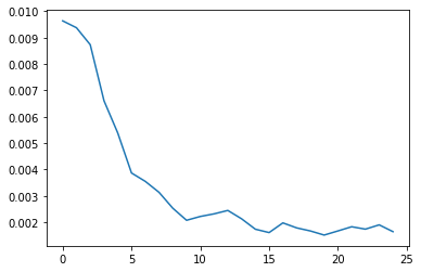
plt.plot(range(len(history.history['loss'])), model.history.history['loss'])
[<matplotlib.lines.Line2D at 0x24121def0c8>]
first_eval_batch = scaled_train[-12:]
first_eval_batch = first_eval_batch.reshape((1, n_input, n_features))
model.predict(first_eval_batch)
array([[0.78138685]], dtype=float32)
Forecast
test_predictions = []
first_eval_batch = scaled_train[-n_input:]
current_batch = first_eval_batch.reshape((1, n_input, n_features))

for i in range(len(test)):
    current_pred = model.predict(current_batch)[0]
    test_predictions.append(current_pred)
    current_batch = np.append(current_batch[:,1:,:], [[current_pred]], axis=1)
test_predictions
[array([0.78138685], dtype=float32),
 array([0.9095711], dtype=float32),
 array([0.85770994], dtype=float32),
 array([1.0188285], dtype=float32),
 array([1.0919129], dtype=float32),
 array([0.84825593], dtype=float32),
 array([1.001781], dtype=float32),
 array([0.87678725], dtype=float32),
 array([0.9534033], dtype=float32),
 array([0.9890802], dtype=float32),
 array([1.060493], dtype=float32),
 array([0.696439], dtype=float32)]
true_predictions = scaler.inverse_transform(test_predictions)
true_predictions
array([[12172.44478464],
       [13672.07242996],
       [13065.34863776],
       [14950.27475297],
       [15805.28861511],
       [12954.74615234],
       [14750.83576441],
       [13288.53398246],
       [14184.86513752],
       [14602.24915051],
       [15437.7075181 ],
       [11178.64018607]])
test['Predictions'] = true_predictions
test
| S4248SM144NCEN | Predictions | |
|---|---|---|
| DATE | ||
| 2018-02-01 | 10415 | 12172.444785 |
| 2018-03-01 | 12683 | 13672.072430 |
| 2018-04-01 | 11919 | 13065.348638 |
| 2018-05-01 | 14138 | 14950.274753 |
| 2018-06-01 | 14583 | 15805.288615 |
| 2018-07-01 | 12640 | 12954.746152 |
| 2018-08-01 | 14257 | 14750.835764 |
| 2018-09-01 | 12396 | 13288.533982 |
| 2018-10-01 | 13914 | 14184.865138 |
| 2018-11-01 | 14174 | 14602.249151 |
| 2018-12-01 | 15504 | 15437.707518 |
| 2019-01-01 | 10718 | 11178.640186 |
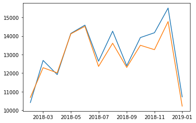
test.plot(figsize=(12,8))
<AxesSubplot:xlabel='DATE'>
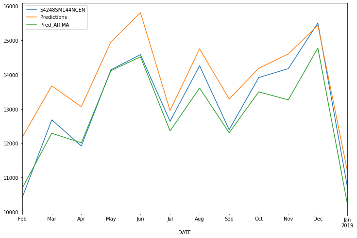
test['Pred_ARIMA'] = pred
print(rmse(test['S4248SM144NCEN'], test['Predictions']))
print(rmse(test['S4248SM144NCEN'], test['Pred_ARIMA']))
873.1015843567056
458.91865971479376