Time Series - Energy Production
Energy Production
import pandas as pd
import numpy as np
import matplotlib.pyplot as plt

from pmdarima import auto_arima
from statsmodels.tsa.holtwinters import ExponentialSmoothing
from sklearn.metrics import mean_squared_error, mean_absolute_error

import warnings
warnings.filterwarnings('ignore')
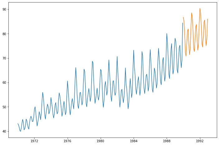
df = pd.read_csv('./Data/EnergyProduction.csv', index_col='DATE', parse_dates=True)
df.plot();
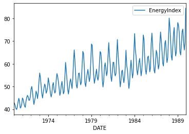
len(df)
240
n_obs = 24
Exponential Smooting
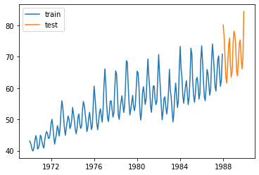
train_data = df.iloc[:-n_obs]
test_data = df.iloc[-n_obs:]
print(train_data.shape, test_data.shape)
(216, 1) (24, 1)
plt.plot(train_data, label='train')
plt.plot(test_data, label='test')
plt.legend()
plt.show()
def exp_smoothing(train_data, trend, seasonal, test_data = test_data):
    fitted_model = ExponentialSmoothing(train_data, trend=trend, seasonal=seasonal,
                                       seasonal_periods=12).fit()
    test_predictions = fitted_model.forecast(24)
    plt.figure(figsize=(12,5))
    plt.plot(test_data, label='test')
    plt.plot(test_predictions, label='prediction')

    mae = mean_absolute_error(test_data, test_predictions)
    mse = mean_squared_error(test_data, test_predictions)
    rmse = np.sqrt(mse)

    print('mae :', mae)
    print('mse :', mse)
    print('rmse :', rmse)
exp_smoothing(train_data, 'mul', 'mul')
mae : 2.7145989390490537
mse : 11.860913777946623
rmse : 3.443967737646017
exp_smoothing(train_data, 'add','add')
mae : 2.768300423888428
mse : 11.775533525016849
rmse : 3.43154972643802
final_model = ExponentialSmoothing(df, trend='add',seasonal='add',
                                  seasonal_periods=12).fit()
forecast_prediction = final_model.forecast(36)
plt.figure(figsize=(12,8))
plt.plot(df)
plt.plot(forecast_prediction)
plt.show()
ARIMA
from statsmodels.tsa.stattools import adfuller
from pmdarima import auto_arima

from statsmodels.tsa.arima_model import ARIMA, ARIMAResults
from statsmodels.tsa.statespace.sarimax import SARIMAX, SARIMAXResults
from statsmodels.graphics.tsaplots import plot_acf, plot_pacf
from statsmodels.tsa.statespace.tools import diff
from statsmodels.tsa.seasonal import seasonal_decompose
from statsmodels.tools.eval_measures import rmse
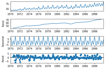
result = seasonal_decompose(df, model='add')
result.plot();
adfuller(df)[1]
0.9830559056338348
df_diff = df.diff().dropna()
adfuller(df_diff)[1]
4.226559012395704e-06
stepwise_fit = auto_arima(df, seasonal=True, trace=True, m=12)
Performing stepwise search to minimize aic
 ARIMA(2,0,2)(1,1,1)[12] intercept   : AIC=842.617, Time=1.00 sec
 ARIMA(0,0,0)(0,1,0)[12] intercept   : AIC=1055.546, Time=0.01 sec
 ARIMA(1,0,0)(1,1,0)[12] intercept   : AIC=855.182, Time=0.15 sec
 ARIMA(0,0,1)(0,1,1)[12] intercept   : AIC=909.065, Time=0.11 sec
 ARIMA(0,0,0)(0,1,0)[12]             : AIC=1134.429, Time=0.01 sec
 ARIMA(2,0,2)(0,1,1)[12] intercept   : AIC=840.759, Time=0.70 sec
 ARIMA(2,0,2)(0,1,0)[12] intercept   : AIC=881.557, Time=0.19 sec
 ARIMA(2,0,2)(0,1,2)[12] intercept   : AIC=842.577, Time=1.42 sec
 ARIMA(2,0,2)(1,1,0)[12] intercept   : AIC=855.194, Time=0.43 sec
 ARIMA(2,0,2)(1,1,2)[12] intercept   : AIC=844.166, Time=1.83 sec
 ARIMA(1,0,2)(0,1,1)[12] intercept   : AIC=841.937, Time=0.28 sec
 ARIMA(2,0,1)(0,1,1)[12] intercept   : AIC=843.582, Time=0.38 sec
 ARIMA(3,0,2)(0,1,1)[12] intercept   : AIC=842.514, Time=0.90 sec
 ARIMA(2,0,3)(0,1,1)[12] intercept   : AIC=842.693, Time=0.94 sec
 ARIMA(1,0,1)(0,1,1)[12] intercept   : AIC=843.610, Time=0.18 sec
 ARIMA(1,0,3)(0,1,1)[12] intercept   : AIC=841.805, Time=0.40 sec
 ARIMA(3,0,1)(0,1,1)[12] intercept   : AIC=840.516, Time=0.75 sec
 ARIMA(3,0,1)(0,1,0)[12] intercept   : AIC=inf, Time=0.44 sec
 ARIMA(3,0,1)(1,1,1)[12] intercept   : AIC=842.397, Time=0.96 sec
 ARIMA(3,0,1)(0,1,2)[12] intercept   : AIC=842.368, Time=1.75 sec
 ARIMA(3,0,1)(1,1,0)[12] intercept   : AIC=855.891, Time=0.67 sec
 ARIMA(3,0,1)(1,1,2)[12] intercept   : AIC=inf, Time=1.87 sec
 ARIMA(3,0,0)(0,1,1)[12] intercept   : AIC=842.621, Time=0.20 sec
 ARIMA(4,0,1)(0,1,1)[12] intercept   : AIC=842.514, Time=0.89 sec
 ARIMA(2,0,0)(0,1,1)[12] intercept   : AIC=844.431, Time=0.16 sec
 ARIMA(4,0,0)(0,1,1)[12] intercept   : AIC=843.014, Time=0.24 sec
 ARIMA(4,0,2)(0,1,1)[12] intercept   : AIC=843.906, Time=0.78 sec
 ARIMA(3,0,1)(0,1,1)[12]             : AIC=843.021, Time=0.51 sec

Best model:  ARIMA(3,0,1)(0,1,1)[12] intercept
Total fit time: 18.180 seconds
stepwise_fit.summary()
| Dep. Variable: | y | No. Observations: | 240 |
|---|---|---|---|
| Model: | SARIMAX(3, 0, 1)x(0, 1, 1, 12) | Log Likelihood | -413.258 |
| Date: | Sun, 23 May 2021 | AIC | 840.516 |
| Time: | 23:55:22 | BIC | 864.522 |
| Sample: | 0 | HQIC | 850.202 |
| - 240 | |||
| Covariance Type: | opg |
| coef | std err | z | P>|z| | [0.025 | 0.975] | |
|---|---|---|---|---|---|---|
| intercept | 0.0475 | 0.046 | 1.044 | 0.296 | -0.042 | 0.137 |
| ar.L1 | 1.6309 | 0.166 | 9.801 | 0.000 | 1.305 | 1.957 |
| ar.L2 | -0.8739 | 0.155 | -5.640 | 0.000 | -1.178 | -0.570 |
| ar.L3 | 0.2156 | 0.091 | 2.376 | 0.017 | 0.038 | 0.394 |
| ma.L1 | -0.7385 | 0.174 | -4.248 | 0.000 | -1.079 | -0.398 |
| ma.S.L12 | -0.5458 | 0.059 | -9.265 | 0.000 | -0.661 | -0.430 |
| sigma2 | 2.1498 | 0.148 | 14.512 | 0.000 | 1.859 | 2.440 |
| Ljung-Box (L1) (Q): | 0.00 | Jarque-Bera (JB): | 64.01 |
|---|---|---|---|
| Prob(Q): | 0.95 | Prob(JB): | 0.00 |
| Heteroskedasticity (H): | 2.07 | Skew: | 0.44 |
| Prob(H) (two-sided): | 0.00 | Kurtosis: | 5.44 |
Warnings:
[1] Covariance matrix calculated using the outer product of gradients (complex-step).
model = SARIMAX(train_data, order=(3,0,1), seasonal_order=(0,1,1,12))
results = model.fit()
results.summary()
| Dep. Variable: | EnergyIndex | No. Observations: | 216 |
|---|---|---|---|
| Model: | SARIMAX(3, 0, 1)x(0, 1, 1, 12) | Log Likelihood | -359.115 |
| Date: | Sun, 23 May 2021 | AIC | 730.230 |
| Time: | 23:56:54 | BIC | 750.138 |
| Sample: | 01-01-1970 | HQIC | 738.283 |
| - 12-01-1987 | |||
| Covariance Type: | opg |
| coef | std err | z | P>|z| | [0.025 | 0.975] | |
|---|---|---|---|---|---|---|
| ar.L1 | 1.7745 | 0.095 | 18.622 | 0.000 | 1.588 | 1.961 |
| ar.L2 | -0.9883 | 0.113 | -8.780 | 0.000 | -1.209 | -0.768 |
| ar.L3 | 0.2111 | 0.076 | 2.778 | 0.005 | 0.062 | 0.360 |
| ma.L1 | -0.8565 | 0.080 | -10.649 | 0.000 | -1.014 | -0.699 |
| ma.S.L12 | -0.5650 | 0.053 | -10.651 | 0.000 | -0.669 | -0.461 |
| sigma2 | 1.9217 | 0.168 | 11.414 | 0.000 | 1.592 | 2.252 |
| Ljung-Box (L1) (Q): | 0.01 | Jarque-Bera (JB): | 9.10 |
|---|---|---|---|
| Prob(Q): | 0.92 | Prob(JB): | 0.01 |
| Heteroskedasticity (H): | 2.05 | Skew: | 0.10 |
| Prob(H) (two-sided): | 0.00 | Kurtosis: | 4.01 |
Warnings:
[1] Covariance matrix calculated using the outer product of gradients (complex-step).
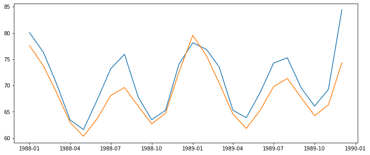
start = len(train_data)
end = len(train_data) + len(test_data) - 1
pred = results.predict(start, end, typ='level')
plt.plot(pred)
plt.plot(test_data)
plt.show()
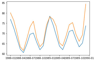
error = rmse(test_data, pred)
error
array([ 8.31981553,  6.09823958,  6.79366971, 10.53638173, 11.99706146,
        8.69493785,  6.05820751,  5.93929791,  7.96124573, 10.79105154,
        9.2213997 ,  6.03056639,  9.51428606,  6.67546108,  6.18212862,
        9.35946757, 10.76244513,  7.70125307,  5.87907598,  5.9064441 ,
        7.08999389,  9.6500675 ,  8.20025993,  6.47869886])
model = SARIMAX(df, order=(3,0,1), seasonal_order=(0,1,1,12))
results = model.fit()
results.summary()
| Dep. Variable: | EnergyIndex | No. Observations: | 240 |
|---|---|---|---|
| Model: | SARIMAX(3, 0, 1)x(0, 1, 1, 12) | Log Likelihood | -415.510 |
| Date: | Sun, 23 May 2021 | AIC | 843.021 |
| Time: | 23:58:43 | BIC | 863.597 |
| Sample: | 01-01-1970 | HQIC | 851.322 |
| - 12-01-1989 | |||
| Covariance Type: | opg |
| coef | std err | z | P>|z| | [0.025 | 0.975] | |
|---|---|---|---|---|---|---|
| ar.L1 | 1.7509 | 0.094 | 18.681 | 0.000 | 1.567 | 1.935 |
| ar.L2 | -0.9646 | 0.117 | -8.235 | 0.000 | -1.194 | -0.735 |
| ar.L3 | 0.2119 | 0.084 | 2.523 | 0.012 | 0.047 | 0.377 |
| ma.L1 | -0.8439 | 0.084 | -10.022 | 0.000 | -1.009 | -0.679 |
| ma.S.L12 | -0.5587 | 0.057 | -9.876 | 0.000 | -0.670 | -0.448 |
| sigma2 | 2.1795 | 0.153 | 14.279 | 0.000 | 1.880 | 2.479 |
| Ljung-Box (L1) (Q): | 0.01 | Jarque-Bera (JB): | 49.80 |
|---|---|---|---|
| Prob(Q): | 0.93 | Prob(JB): | 0.00 |
| Heteroskedasticity (H): | 2.08 | Skew: | 0.40 |
| Prob(H) (two-sided): | 0.00 | Kurtosis: | 5.14 |
Warnings:
[1] Covariance matrix calculated using the outer product of gradients (complex-step).
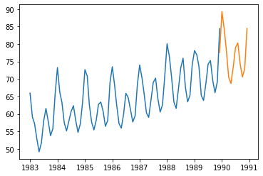
forecast = results.predict(len(df)-1, len(df)+11, typ='levels')
plt.plot(df['1983-01-01':])
plt.plot(forecast)
[<matplotlib.lines.Line2D at 0x14301670908>]
LSTM
from tensorflow.keras.preprocessing.sequence import TimeseriesGenerator
from sklearn.preprocessing import MinMaxScaler, StandardScaler
from tensorflow.keras.models import Model
from tensorflow.keras.layers import Dense, LSTM, Input
nobs = 12
train = df.iloc[:-nobs]
test = df.iloc[-nobs:]
mm_scaler = MinMaxScaler()
st_scaler = StandardScaler()
mm_scaler.fit(train)
st_scaler.fit(train)
StandardScaler()
mm_scaled_train = mm_scaler.transform(train)
mm_scaled_test = mm_scaler.transform(test)
st_scaled_train = st_scaler.transform(train)
st_scaled_test = st_scaler.transform(test)
n_input = 12
n_features = 1
mm_gen = TimeseriesGenerator(mm_scaled_train, mm_scaled_train, length=n_input,
                         batch_size=1)
st_gen = TimeseriesGenerator(st_scaled_train, st_scaled_train, length=n_input,
                         batch_size=1)
inputs = Input(shape=(n_input, n_features))
x = LSTM(100, activation='relu')(inputs)
x = Dense(1)(x)
WARNING:tensorflow:Layer lstm will not use cuDNN kernel since it doesn't meet the cuDNN kernel criteria. It will use generic GPU kernel as fallback when running on GPU
mm_model = Model(inputs, x)
st_model = Model(inputs, x)
mm_model.compile(optimizer='adam', loss='mse')
st_model.compile(optimizer='adam', loss='mse')
mm_hist = mm_model.fit_generator(mm_gen, epochs=50, verbose=0)
st_hist = st_model.fit_generator(st_gen, epochs=50, verbose=0)
WARNING:tensorflow:From <ipython-input-23-6ebd85666877>:1: Model.fit_generator (from tensorflow.python.keras.engine.training) is deprecated and will be removed in a future version.
Instructions for updating:
Please use Model.fit, which supports generators.
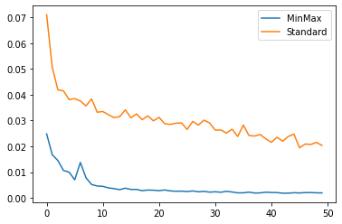
plt.plot(mm_hist.history['loss'], label='MinMax')
plt.plot(st_hist.history['loss'], label='Standard')
plt.legend()
plt.show()
first_eval_batch = mm_scaled_train[-12:]
first_eval_batch = first_eval_batch.reshape((1, n_input, n_features))
mm_model.predict(first_eval_batch)
array([[1.1262071]], dtype=float32)
test_predictions = []
first_eval_batch = mm_scaled_train[-n_input:]
current_batch = first_eval_batch.reshape((1, n_input, n_features))
for i in range(len(test)):
    current_pred = model.predict(current_batch)[0]
    test_predictions.append(current_pred)
    current_batch = np.append(current_batch[:, 1:, :], [[current_pred]], axis=1)
test_predictions
[array([1.1262071], dtype=float32),
 array([1.117718], dtype=float32),
 array([0.83300537], dtype=float32),
 array([0.5422754], dtype=float32),
 array([0.5601636], dtype=float32),
 array([0.8953703], dtype=float32),
 array([1.2141159], dtype=float32),
 array([1.146272], dtype=float32),
 array([0.80624], dtype=float32),
 array([0.52206135], dtype=float32),
 array([0.63773364], dtype=float32),
 array([1.1513337], dtype=float32)]
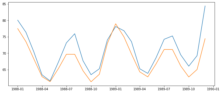
true_predictions = mm_scaler.inverse_transform(test_predictions)
test['predictions'] = true_predictions
test.plot(figsize=(12,9))
<AxesSubplot:xlabel='DATE'>
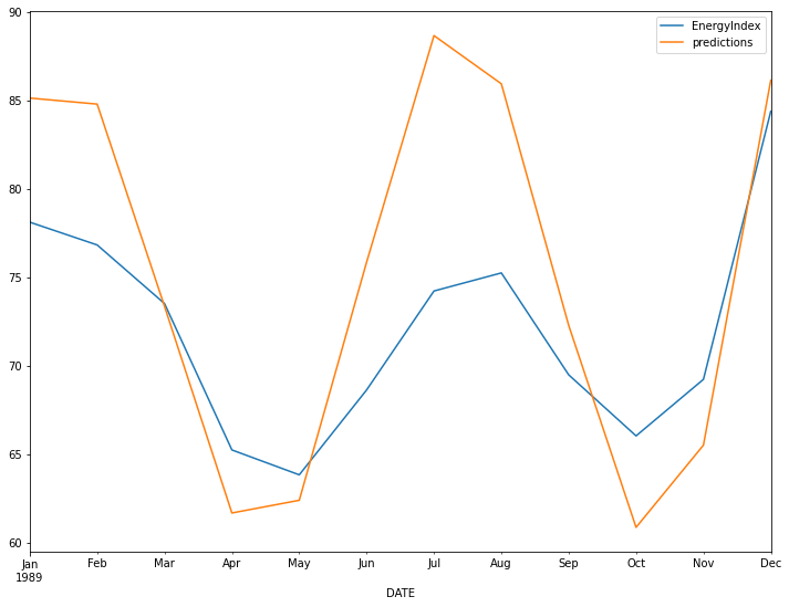
print(rmse(test['EnergyIndex'], test['predictions']))
6.790834064681344