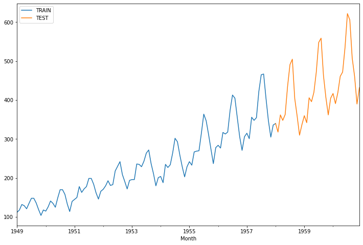
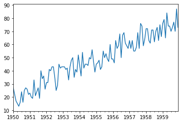
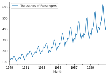
<class 'pandas.core.frame.DataFrame'>
DatetimeIndex: 144 entries, 1949-01-01 to 1960-12-01
Freq: MS
Data columns (total 1 columns):
 #   Column                   Non-Null Count  Dtype
---  ------                   --------------  -----
 0   Thousands of Passengers  144 non-null    int64
dtypes: int64(1)
memory usage: 2.2 KB
C:\Users\ilvna\.conda\envs\tf-2.3\lib\site-packages\statsmodels\tsa\holtwinters\model.py:429: FutureWarning: After 0.13 initialization must be handled at model creation
  FutureWarning,
C:\Users\ilvna\.conda\envs\tf-2.3\lib\site-packages\statsmodels\tsa\holtwinters\model.py:80: RuntimeWarning: overflow encountered in matmul
  return err.T @ err
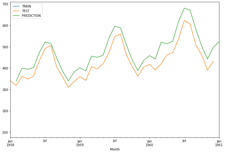
1958-02-01    339.142839
1958-03-01    399.281567
1958-04-01    394.233518
1958-05-01    402.545212
1958-06-01    473.128729
1958-07-01    521.795258
1958-08-01    514.513564
1958-09-01    446.216722
1958-10-01    385.430842
1958-11-01    339.645012
1958-12-01    381.455551
1959-01-01    401.210071
1959-02-01    387.159060
1959-03-01    455.812296
1959-04-01    450.049538
1959-05-01    459.538011
1959-06-01    540.114821
1959-07-01    595.671611
1959-08-01    587.358966
1959-09-01    509.392582
1959-10-01    440.000570
1959-11-01    387.732331
1959-12-01    435.462452
1960-01-01    458.013840
1960-02-01    441.973470
1960-03-01    520.346708
1960-04-01    513.768052
1960-05-01    524.599914
1960-06-01    616.584878
1960-07-01    680.007460
1960-08-01    670.517902
1960-09-01    581.512951
1960-10-01    502.296340
1960-11-01    442.627906
1960-12-01    497.115710
1961-01-01    522.859949
Freq: MS, dtype: float64
<AxesSubplot:xlabel='Month'>
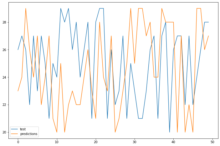
train_data['Thousands of Passengers'].plot(legend=True, label='TRAIN',figsize=(12,8))
test_data['Thousands of Passengers'].plot(legend=True, label='TEST')
test_predictions.plot(legend=True, label='PREDICTION',xlim=['1958-01-01','1961-01-01'])
<AxesSubplot:xlabel='Month'>
C:\Users\ilvna\.conda\envs\tf-2.3\lib\site-packages\statsmodels\tsa\holtwinters\model.py:429: FutureWarning: After 0.13 initialization must be handled at model creation
  FutureWarning,
C:\Users\ilvna\.conda\envs\tf-2.3\lib\site-packages\statsmodels\tsa\holtwinters\model.py:80: RuntimeWarning: overflow encountered in matmul
  return err.T @ err
<AxesSubplot:xlabel='Month'>
array([ 1. , -0.5 , -0.2 , 0.275, -0.075])
array([ 1. , -0.625 , -1.18803419, 2.03764205, 0.8949589 ])
array([ 1. , -0.49677419, -0.43181818, 0.53082621, 0.25434783])
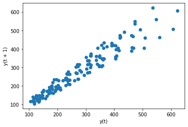
<AxesSubplot:xlabel='y(t)', ylabel='y(t + 1)'>
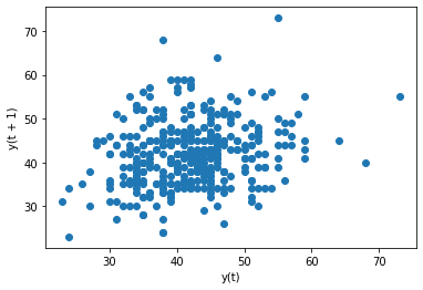
<AxesSubplot:xlabel='y(t)', ylabel='y(t + 1)'>
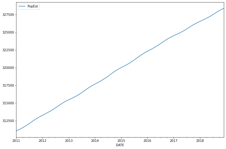
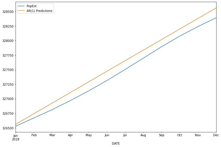
<AxesSubplot:xlabel='DATE'>
const        284.913797
L1.PopEst      0.999686
dtype: float64
2018-01-01    326560.403377
2018-02-01    326742.749463
2018-03-01    326925.038278
2018-04-01    327107.269838
2018-05-01    327289.444162
2018-06-01    327471.561268
2018-07-01    327653.621173
2018-08-01    327835.623896
2018-09-01    328017.569455
2018-10-01    328199.457868
2018-11-01    328381.289152
2018-12-01    328563.063326
Freq: MS, dtype: float64
2018-01-01    326560.403377
2018-02-01    326742.749463
2018-03-01    326925.038278
2018-04-01    327107.269838
2018-05-01    327289.444162
2018-06-01    327471.561268
2018-07-01    327653.621173
2018-08-01    327835.623896
2018-09-01    328017.569455
2018-10-01    328199.457868
2018-11-01    328381.289152
2018-12-01    328563.063326
Freq: MS, Name: AR(1) Predictions, dtype: float64
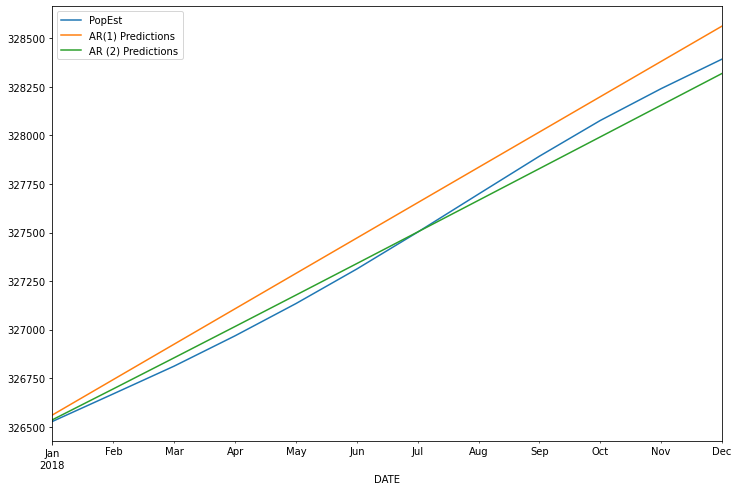
<AxesSubplot:xlabel='DATE'>
const        137.368305
L1.PopEst      1.853490
L2.PopEst     -0.853836
dtype: float64
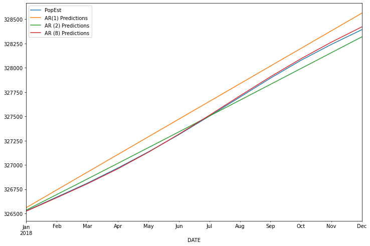
<AxesSubplot:xlabel='DATE'>
const        82.309677
L1.PopEst     2.437997
L2.PopEst    -2.302100
L3.PopEst     1.565427
L4.PopEst    -1.431211
L5.PopEst     1.125022
L6.PopEst    -0.919494
L7.PopEst     0.963694
L8.PopEst    -0.439511
dtype: float64
AR1 MSE was : 17449.714239577344
AR2 MSE was : 2713.258615675103
AR8 MSE was : 186.97377437908688
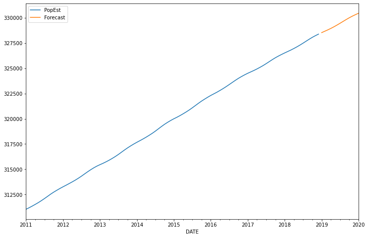
<AxesSubplot:xlabel='DATE'>
<AxesSubplot:xlabel='DATE'>
<AxesSubplot:xlabel='Month'>
(0.8153688792060512,
 0.991880243437641,
 13,
 130,
 {'1%': -3.4816817173418295,
  '5%': -2.8840418343195267,
  '10%': -2.578770059171598},
 996.692930839019)
Help on function adfuller in module statsmodels.tsa.stattools:

adfuller(x, maxlag=None, regression='c', autolag='AIC', store=False, regresults=False)
    Augmented Dickey-Fuller unit root test.

    The Augmented Dickey-Fuller test can be used to test for a unit root in a
    univariate process in the presence of serial correlation.

    Parameters
    ----------
    x : array_like, 1d
        The data series to test.
    maxlag : int
        Maximum lag which is included in test, default 12*(nobs/100)^{1/4}.
    regression : {"c","ct","ctt","nc"}
        Constant and trend order to include in regression.

        * "c" : constant only (default).
        * "ct" : constant and trend.
        * "ctt" : constant, and linear and quadratic trend.
        * "nc" : no constant, no trend.

    autolag : {"AIC", "BIC", "t-stat", None}
        Method to use when automatically determining the lag.

        * if None, then maxlag lags are used.
        * if "AIC" (default) or "BIC", then the number of lags is chosen
          to minimize the corresponding information criterion.
        * "t-stat" based choice of maxlag.  Starts with maxlag and drops a
          lag until the t-statistic on the last lag length is significant
          using a 5%-sized test.
    store : bool
        If True, then a result instance is returned additionally to
        the adf statistic. Default is False.
    regresults : bool, optional
        If True, the full regression results are returned. Default is False.

    Returns
    -------
    adf : float
        The test statistic.
    pvalue : float
        MacKinnon"s approximate p-value based on MacKinnon (1994, 2010).
    usedlag : int
        The number of lags used.
    nobs : int
        The number of observations used for the ADF regression and calculation
        of the critical values.
    critical values : dict
        Critical values for the test statistic at the 1 %, 5 %, and 10 %
        levels. Based on MacKinnon (2010).
    icbest : float
        The maximized information criterion if autolag is not None.
    resstore : ResultStore, optional
        A dummy class with results attached as attributes.

    Notes
    -----
    The null hypothesis of the Augmented Dickey-Fuller is that there is a unit
    root, with the alternative that there is no unit root. If the pvalue is
    above a critical size, then we cannot reject that there is a unit root.

    The p-values are obtained through regression surface approximation from
    MacKinnon 1994, but using the updated 2010 tables. If the p-value is close
    to significant, then the critical values should be used to judge whether
    to reject the null.

    The autolag option and maxlag for it are described in Greene.

    References
    ----------
    .. [1] W. Green.  "Econometric Analysis," 5th ed., Pearson, 2003.

    .. [2] Hamilton, J.D.  "Time Series Analysis".  Princeton, 1994.

    .. [3] MacKinnon, J.G. 1994.  "Approximate asymptotic distribution functions for
        unit-root and cointegration tests.  `Journal of Business and Economic
        Statistics` 12, 167-76.

    .. [4] MacKinnon, J.G. 2010. "Critical Values for Cointegration Tests."  Queen"s
        University, Dept of Economics, Working Papers.  Available at
        http://ideas.repec.org/p/qed/wpaper/1227.html

    Examples
    --------
    See example notebook
ADF Test Statistic        0.815369
p-value                   0.991880
# Lags Used              13.000000
# Observations          130.000000
critical value (1%)      -3.481682
critical value (5%)      -2.884042
critical value (10%)     -2.578770
dtype: float64
from statsmodels.tsa.stattools import adfuller

def adf_test(series, title=''):
    """
    Pass in a time series and an optional title, returns an ADF report
    """
    print(f'Augmented Dickey-Fuller Test: {title}')
    result = adfuller(series.dropna(), autolag = 'AIC')

    labels = ['ADF test statistic', 'p-value', '# lags used', '# obervations']
    out = pd.Series(result[0:4], index = labels)

    for key, val in result[4].items():
        out[f'critical value ({key})'] = val

    print(out.to_string())

    if result[1] <= 0.05:
        print('Strong evidence against the null hypothesis')
        print('Reject the null hypothesis')
        print('Data has no unit root and is stationary')
    else:
        print('Weak evidence against the null hypothesis')
        print('Fail to reject the null hypothesis')
        print('Data has a unit root and is non-stationary')
Augmented Dickey-Fuller Test:
ADF test statistic        0.815369
p-value                   0.991880
# lags used              13.000000
# obervations           130.000000
critical value (1%)      -3.481682
critical value (5%)      -2.884042
critical value (10%)     -2.578770
Weak evidence against the null hypothesis
Fail to reject the null hypothesis
Data has a unit root and is non-stationary
<AxesSubplot:xlabel='Month'>
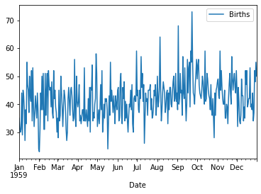
<AxesSubplot:xlabel='Date'>
Augmented Dickey-Fuller Test:
ADF test statistic       -4.808291
p-value                   0.000052
# lags used               6.000000
# obervations           358.000000
critical value (1%)      -3.448749
critical value (5%)      -2.869647
critical value (10%)     -2.571089
Strong evidence against the null hypothesis
Reject the null hypothesis
Data has no unit root and is stationary
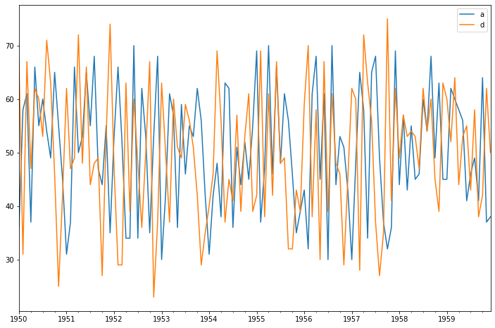
Granger Causality
number of lags (no zero) 1
ssr based F test: F=1.7051 , p=0.1942 , df_denom=116, df_num=1
ssr based chi2 test: chi2=1.7492 , p=0.1860 , df=1
likelihood ratio test: chi2=1.7365 , p=0.1876 , df=1
parameter F test: F=1.7051 , p=0.1942 , df_denom=116, df_num=1
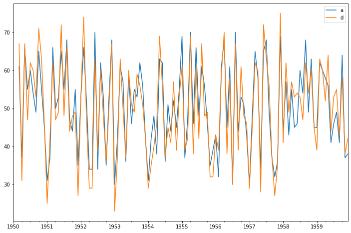
Granger Causality
number of lags (no zero) 2
ssr based F test: F=286.0339, p=0.0000 , df_denom=113, df_num=2
ssr based chi2 test: chi2=597.3806, p=0.0000 , df=2
likelihood ratio test: chi2=212.6514, p=0.0000 , df=2
parameter F test: F=286.0339, p=0.0000 , df_denom=113, df_num=2
Granger Causality
number of lags (no zero) 3
ssr based F test: F=188.7446, p=0.0000 , df_denom=110, df_num=3
ssr based chi2 test: chi2=602.2669, p=0.0000 , df=3
likelihood ratio test: chi2=212.4789, p=0.0000 , df=3
parameter F test: F=188.7446, p=0.0000 , df_denom=110, df_num=3
Granger Causality
number of lags (no zero) 1
ssr based F test:         F=1.5225  , p=0.2197  , df_denom=116, df_num=1
ssr based chi2 test:   chi2=1.5619  , p=0.2114  , df=1
likelihood ratio test: chi2=1.5517  , p=0.2129  , df=1
parameter F test:         F=1.5225  , p=0.2197  , df_denom=116, df_num=1

Granger Causality
number of lags (no zero) 2
ssr based F test:         F=0.4350  , p=0.6483  , df_denom=113, df_num=2
ssr based chi2 test:   chi2=0.9086  , p=0.6349  , df=2
likelihood ratio test: chi2=0.9051  , p=0.6360  , df=2
parameter F test:         F=0.4350  , p=0.6483  , df_denom=113, df_num=2

Granger Causality
number of lags (no zero) 3
ssr based F test:         F=0.5333  , p=0.6604  , df_denom=110, df_num=3
ssr based chi2 test:   chi2=1.7018  , p=0.6365  , df=3
likelihood ratio test: chi2=1.6895  , p=0.6393  , df=3
parameter F test:         F=0.5333  , p=0.6604  , df_denom=110, df_num=3
17.02
4.125530268947253
3.54
<AxesSubplot:xlabel='Month'>