LSTM Autoencoder for Anomaly Detection
LSTM Autoencoder for Anomaly Detection
- 정상적인 데이터로 모델 학습 후 비정상적인 데이터를 넣어 디코딩하게 되면 정상 데이터 특성과 디코딩 된 데이터 간의 차이인 재구성 손실(Reconstruction Error)를 계산하여 손실이 낮은 부분은 normal, 높은 부분은 abnormal로 판단
- Sequence data에 Encoder-Decoder LSTM Architecture를 적용하여 구현. Model에 input sequence가 순차적으로 들어오게 되고, 마지막 input sequence가 들어온 후 decoder는 input sequence를 재생성하거나 목표 sequence에 대한 예측을 출력.
- LSTM Autoencoder 학습 시 normal data로만 학습.
LSTM Autoencoder through Curve shifting
Curve Shifting을 통해 데이터의 시점을 변환해주고 normal 데이터만을 통해 LSTM AE모델을 학습. 그 후 재구성 손실을 계산 후 Precision Recall Curve를 통해 normal/abnormal을 구분하기 위한 threshold를 지정하고 이를 기준으로 test set의 재구성 손실을 분류하여 t+n 시점을 예측.
1. Curve Shifting
사전 예측 개념을 적용하기 위한 Shifting 방법. 비정상 신호를 n일 전에 조기예측 하고자 한다면 n일 만큼 shift하는게 아니라 비정상 신호가 있는 날짜로부터 n일 전까지의 데이터를 비정상 신호로 바꾸어 주는것. 그후 본래 비정상 신호 데이터를 제거해주는데 라벨을 바꿔주는 순간 비정상 신호 예측 문제가 아닌 비정상 신호 조짐 예측 문제가 되는것이기 때문에 데이터의 학습혼동을 없애주기 위해 제거.
2. Threshold by Precision-Recall-Curve
적절한 Threshold값을 적용하기 위한 방법. Recall과 Precision이 서로 Trade off 관계를 가지기 때문에 어느 한쪽에 치우치지 않는 최적의 threshold를 구하기 위한 방법.
Implementation
Imports
import pandas as pd
import numpy as np
import matplotlib.pyplot as plt
import seaborn as sns
from pylab import rcParams
from collections import Counter
import os

import tensorflow as tf
from tensorflow.keras.models import Model
from tensorflow.keras.layers import Input, LSTM, RepeatVector, TimeDistributed, Dense
from tensorflow.keras.optimizers import Adam
from tensorflow.keras.callbacks import EarlyStopping
from tensorflow.keras.utils import plot_model

from sklearn.preprocessing import StandardScaler
from sklearn.model_selection import train_test_split
from sklearn import metrics
import tensorboard
from datetime import datetime

import warnings
warnings.filterwarnings('ignore')
Dataset
LABELS = ['Normal', 'Break']
df = pd.read_excel('./processminer-rare-event-mts.xlsx', engine='openpyxl')
df.shape
(18398, 63)
Counter(df['y'])
Counter({0: 18274, 1: 124})
Curve Shifting
sign = lambda x: (1, -1)[x < 0]
def curve_shift(df, shift_by):
    vector = df['y'].copy()
    for _ in range(abs(shift_by)):
        tmp = vector.shift(sign(shift_by))
        tmp = tmp.fillna(0)
        vector += tmp
    labelcol = 'y'

    # Add vector to the df
    df.insert(loc=0, column=labelcol+'tmp', value=vector)

    # Remove the rows with labelcol == 1
    df = df.drop(df[df[labelcol]==1].index)

    df = df.drop(labelcol, axis=1)
    df = df.rename(columns={labelcol+'tmp': labelcol})

    df.loc[df[labelcol] > 0, labelcol] = 1

    return df
shifted_df = curve_shift(df, shift_by=-5)
shifted_df.head()
| y | time | x1 | x2 | x3 | x4 | x5 | x6 | x7 | x8 | ... | x52 | x53 | x54 | x55 | x56 | x57 | x58 | x59 | x60 | x61 | |
|---|---|---|---|---|---|---|---|---|---|---|---|---|---|---|---|---|---|---|---|---|---|
| 0 | 0.0 | 1999-05-01 00:00:00 | 0.376665 | -4.596435 | -4.095756 | 13.497687 | -0.118830 | -20.669883 | 0.000732 | -0.061114 | ... | 10.091721 | 0.053279 | -4.936434 | -24.590146 | 18.515436 | 3.473400 | 0.033444 | 0.953219 | 0.006076 | 0 |
| 1 | 0.0 | 1999-05-01 00:02:00 | 0.475720 | -4.542502 | -4.018359 | 16.230659 | -0.128733 | -18.758079 | 0.000732 | -0.061114 | ... | 10.095871 | 0.062801 | -4.937179 | -32.413266 | 22.760065 | 2.682933 | 0.033536 | 1.090502 | 0.006083 | 0 |
| 2 | 0.0 | 1999-05-01 00:04:00 | 0.363848 | -4.681394 | -4.353147 | 14.127997 | -0.138636 | -17.836632 | 0.010803 | -0.061114 | ... | 10.100265 | 0.072322 | -4.937924 | -34.183774 | 27.004663 | 3.537487 | 0.033629 | 1.840540 | 0.006090 | 0 |
| 3 | 0.0 | 1999-05-01 00:06:00 | 0.301590 | -4.758934 | -4.023612 | 13.161566 | -0.148142 | -18.517601 | 0.002075 | -0.061114 | ... | 10.104660 | 0.081600 | -4.938669 | -35.954281 | 21.672449 | 3.986095 | 0.033721 | 2.554880 | 0.006097 | 0 |
| 4 | 0.0 | 1999-05-01 00:08:00 | 0.265578 | -4.749928 | -4.333150 | 15.267340 | -0.155314 | -17.505913 | 0.000732 | -0.061114 | ... | 10.109054 | 0.091121 | -4.939414 | -37.724789 | 21.907251 | 3.601573 | 0.033777 | 1.410494 | 0.006105 | 0 |
5 rows × 63 columns
shifted_df = shifted_df.drop(['time', 'x28','x61'], axis=1)
input_x = shifted_df.drop('y', axis=1).values
input_y = shifted_df['y'].values
n_features = input_x.shape[1]
def temporalize(X, y, timesteps):
    output_X = []
    output_y = []
    for i in range(len(X) - timesteps -1):
        t = []
        for j in range(1, timesteps + 1):
            t.append(X[[(i+j+1)], :])
        output_X.append(t)
        output_y.append(y[i+timesteps+1])
    return np.squeeze(np.array(output_X)), np.array(output_y)
timesteps = 5
x, y = temporalize(input_x, input_y, timesteps)
print(x.shape)
(18268, 5, 59)
Trian Test Split
x_train, x_test, y_train, y_test = train_test_split(x, y, test_size=.2)
x_train, x_valid, y_train, y_valid = train_test_split(x_train, y_train, test_size=.2)

print(len(x_train))
print(len(x_valid))
print(len(x_test))
11691
2923
3654
Normal(0) / Break(1) data split
x_train_y0 = x_train[y_train == 0]
x_train_y1 = x_train[y_train == 1]

x_valid_y0 = x_valid[y_valid == 0]
x_valid_y1 = x_valid[y_valid == 1]
Standardize
def flatten(X):
    flattened_X = np.empty((X.shape[0], X.shape[2]))
    for i in range(X.shape[0]):
        flattened_X[i] = X[i, (X.shape[1]-1), :]
    return(flattened_X)

def scale(X, scaler):
    for i in range(X.shape[0]):
        X[i, :, :] = scaler.transform(X[i, :, :])

    return X
scaler = StandardScaler().fit(flatten(x_train_y0))

x_train_y0_scaled = scale(x_train_y0, scaler)
x_valid_scaled = scale(x_valid, scaler)
x_valid_y0_scaled = scale(x_valid_y0, scaler)
x_test_scaled = scale(x_test, scaler)
Model
epochs = 200
batch = 128
lr = 0.001
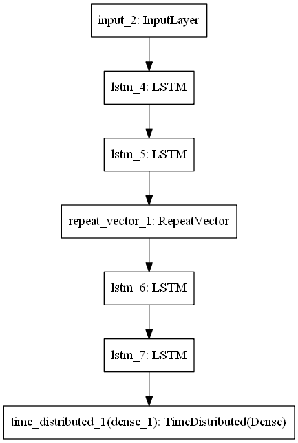
inputs = Input(shape=(timesteps, n_features))
# Encoder
x = LSTM(32, activation='tanh', return_sequences=True)(inputs)
x = LSTM(16, activation='tanh', return_sequences=False)(x)
x = RepeatVector(timesteps)(x)

# Decoder
x = LSTM(16, activation='tanh', return_sequences=True)(x)
x = LSTM(32, activation='tanh', return_sequences=True)(x)
x = TimeDistributed(Dense(n_features))(x)

model = Model(inputs, x)
model.summary()
Model: "functional_3"
_________________________________________________________________
Layer (type)                 Output Shape              Param #
=================================================================
input_2 (InputLayer)         [(None, 5, 59)]           0
_________________________________________________________________
lstm_4 (LSTM)                (None, 5, 32)             11776
_________________________________________________________________
lstm_5 (LSTM)                (None, 16)                3136
_________________________________________________________________
repeat_vector_1 (RepeatVecto (None, 5, 16)             0
_________________________________________________________________
lstm_6 (LSTM)                (None, 5, 16)             2112
_________________________________________________________________
lstm_7 (LSTM)                (None, 5, 32)             6272
_________________________________________________________________
time_distributed_1 (TimeDist (None, 5, 59)             1947
=================================================================
Total params: 25,243
Trainable params: 25,243
Non-trainable params: 0
_________________________________________________________________
plot_model(model)
model.compile(loss='mse', optimizer = Adam(lr))
logdir = 'log/LSTMAE/'+datetime.now().strftime("%Y%m%d-%H%M%S")
tensorboard_callback = tf.keras.callbacks.TensorBoard(log_dir = logdir)
es = EarlyStopping(monitor='val_loss', patience=5)
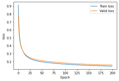
history = model.fit(x_train_y0_scaled, x_train_y0_scaled,
                   epochs = epochs, batch_size = batch,
                   validation_data=(x_valid_y0_scaled, x_valid_y0_scaled), callbacks=[tensorboard_callback, es], verbose=0)
WARNING:tensorflow:Callbacks method `on_train_batch_end` is slow compared to the batch time (batch time: 0.0070s vs `on_train_batch_end` time: 0.1635s). Check your callbacks.
plt.plot(history.history['loss'], label='Train loss')
plt.plot(history.history['val_loss'], label='Valid loss')
plt.legend()
plt.xlabel('Epoch')
plt.ylabel('loss')
plt.show()
Threshold by Precision Recall Curve
valid_x_predictions = model.predict(x_valid_scaled)
mse = np.mean(np.power(flatten(x_valid_scaled) - flatten(valid_x_predictions),
                      2,), axis=1)

error_df = pd.DataFrame({'Reconstruction_error' : mse,
                        'True_class' : list(y_valid)})
precision_rt, recall_rt, threshold_rt = metrics.precision_recall_curve(error_df['True_class'], error_df['Reconstruction_error'])

plt.figure(figsize=(8,5))
plt.plot(threshold_rt, precision_rt[1:], label='Precision')
plt.plot(threshold_rt, recall_rt[1:], label='Recall')
plt.xlabel('Threshold')
plt.ylabel('Precision/Recall')
plt.legend()
plt.show()
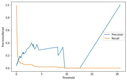
index_cnt = [cnt for cnt, (p, r) in enumerate(zip(precision_rt, recall_rt)) if p==r][0]
print('Precision: ',precision_rt[index_cnt],', Recall: ', recall_rt[index_cnt])

threshold_fixed = threshold_rt[index_cnt]
print('Threshold: ', threshold_fixed)
Precision:  0.13636363636363635 , Recall:  0.13636363636363635
Threshold:  0.40606808904917024
Best threshold : 0.403
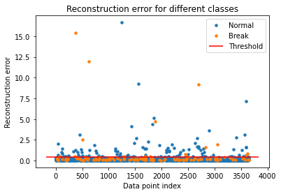
Predict Test
test_x_predictions = model.predict(x_test_scaled)
mse = np.mean(np.power(flatten(x_test_scaled) - flatten(test_x_predictions), 2), axis=1)

error_df = pd.DataFrame({'Reconstruction_error': mse,
                        'True_class' : y_test.tolist()})

groups = error_df.groupby('True_class')
fig, ax = plt.subplots()

for name, group in groups:
    ax.plot(group.index, group.Reconstruction_error, marker='o', ms=3.5, linestyle='',
            label= "Break" if name == 1 else "Normal")
ax.hlines(threshold_fixed, ax.get_xlim()[0], ax.get_xlim()[1], colors="r", zorder=100, label='Threshold')
ax.legend()
plt.title("Reconstruction error for different classes")
plt.ylabel("Reconstruction error")
plt.xlabel("Data point index")
plt.show();
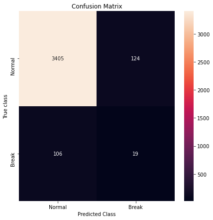
Confusion Matrix
pred_y = [1 if e > threshold_fixed else 0 for e in error_df['Reconstruction_error'].values]

cm = metrics.confusion_matrix(error_df['True_class'], pred_y)
plt.figure(figsize=(7,7))
sns.heatmap(cm, xticklabels=LABELS, yticklabels=LABELS, annot=True, fmt='d')
plt.title('Confusion Matrix')
plt.xlabel('Predicted Class')
plt.ylabel('True class')
plt.show()
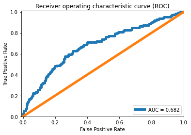
ROC curve
false_pos_rate, true_pos_rate, thresholds = metrics.roc_curve(error_df['True_class'], error_df['Reconstruction_error'])
roc_auc = metrics.auc(false_pos_rate, true_pos_rate,)

plt.plot(false_pos_rate, true_pos_rate, linewidth=5, label='AUC = %0.3f'% roc_auc)
plt.plot([0,1],[0,1], linewidth=5)

plt.xlim([-0.01, 1])
plt.ylim([0, 1.01])
plt.legend(loc='lower right')
plt.title('Receiver operating characteristic curve (ROC)')
plt.ylabel('True Positive Rate'); plt.xlabel('False Positive Rate')
plt.show()
Reference
- https://towardsdatascience.com/extreme-rare-event-classification-using-autoencoders-in-keras-a565b386f098
- https://towardsdatascience.com/lstm-autoencoder-for-extreme-rare-event-classification-in-keras-ce209a224cfb