Time Series of Price Anomaly Detection with LSTM
Time Series of Price Anomaly Detection with LSTM
from sklearn.preprocessing import StandardScaler
import matplotlib.pyplot as plt
import pandas as pd
import numpy as np

from tensorflow.keras.models import Model
from tensorflow.keras.layers import Dense, LSTM, Dropout, RepeatVector, TimeDistributed
from tensorflow.keras.layers import Input
from tensorflow.keras.callbacks import EarlyStopping


import warnings
warnings.filterwarnings('ignore')
Dataset
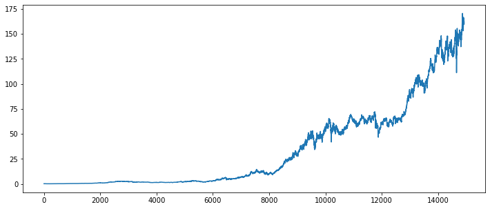
df = pd.read_csv('JNJ.csv')
df = df[['Date','Close']]
df['Date'] = pd.to_datetime(df['Date'])
plt.figure(figsize=(12,5))
plt.plot(df['Close'])
plt.show()
Preprocessing
train, test = df.loc[:11940], df.loc[11941:]
scaler = StandardScaler()
scaler = scaler.fit(train[['Close']])
train['Close'] = scaler.transform(train[['Close']])
test['Close'] = scaler.transform(test[['Close']])
TIME_STEPS = 30
def create_sequences(X, y, time_steps = TIME_STEPS):
    Xs, ys = [], []
    for i in range(len(X)-time_steps):
        Xs.append(X.iloc[i:(i+time_steps)].values)
        ys.append(y.iloc[i+time_steps])

    return np.array(Xs), np.array(ys)
X_train, y_train = create_sequences(train[['Close']], train['Close'])
X_test, y_test = create_sequences(test[['Close']], test['Close'])
print(train.shape)
(11941, 2)
print(X_train.shape)
(11911, 30, 1)
Model
print(X_train.shape[1])
print(X_train.shape[2])
30
1
inputs = Input(shape = (X_train.shape[1], X_train.shape[2]))
x = LSTM(128)(inputs)
x = Dropout(rate=0.2)(x)
x = RepeatVector(X_train.shape[1])(x)

x = LSTM(128, return_sequences = True)(x)
x = Dropout(rate=0.2)(x)
# ###
# x = LSTM(128, return_sequences = True)(x)
# x = Dropout(rate=0.2)(x)
# ###

x = TimeDistributed(Dense(X_train.shape[2]))(x)
model = Model(inputs, x)
model.compile(optimizer='adam', loss='mse')
model.summary()
Model: "functional_1"
_________________________________________________________________
Layer (type)                 Output Shape              Param #
=================================================================
input_1 (InputLayer)         [(None, 30, 1)]           0
_________________________________________________________________
lstm (LSTM)                  (None, 128)               66560
_________________________________________________________________
dropout (Dropout)            (None, 128)               0
_________________________________________________________________
repeat_vector (RepeatVector) (None, 30, 128)           0
_________________________________________________________________
lstm_1 (LSTM)                (None, 30, 128)           131584
_________________________________________________________________
dropout_1 (Dropout)          (None, 30, 128)           0
_________________________________________________________________
time_distributed (TimeDistri (None, 30, 1)             129
=================================================================
Total params: 198,273
Trainable params: 198,273
Non-trainable params: 0
_________________________________________________________________
es = EarlyStopping(monitor='val_loss', patience=3, mode='min')
hist = model.fit(X_train, y_train, epochs=100, batch_size=32,
                validation_split=0.2,
                callbacks=[es], shuffle=False)
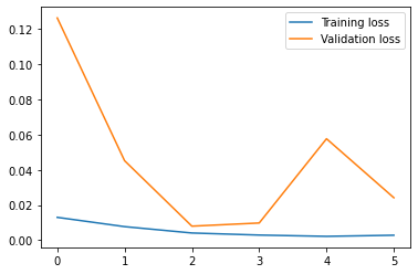
Epoch 1/100
298/298 [==============================] - 2s 8ms/step - loss: 0.0130 - val_loss: 0.1263
Epoch 2/100
298/298 [==============================] - 2s 6ms/step - loss: 0.0077 - val_loss: 0.0452
Epoch 3/100
298/298 [==============================] - 2s 6ms/step - loss: 0.0041 - val_loss: 0.0080
Epoch 4/100
298/298 [==============================] - 2s 6ms/step - loss: 0.0029 - val_loss: 0.0098
Epoch 5/100
298/298 [==============================] - 2s 6ms/step - loss: 0.0022 - val_loss: 0.0576
Epoch 6/100
298/298 [==============================] - 2s 6ms/step - loss: 0.0028 - val_loss: 0.0241
plt.plot(hist.history['loss'], label='Training loss')
plt.plot(hist.history['val_loss'], label='Validation loss')
plt.legend()
plt.show()
Anomalies
X_train_pred = model.predict(X_train, verbose=0)
train_mae_loss = np.mean(np.abs(X_train_pred - X_train), axis=1)
plt.hist(train_mae_loss, bins=50)
plt.xlabel('Train MAE loss')
plt.ylabel('Number of Samples')
plt.show()
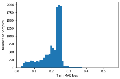
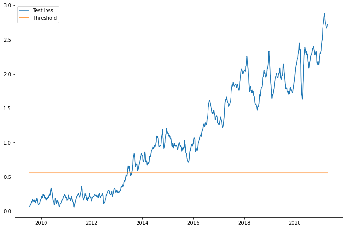
threshold = np.max(train_mae_loss)
print(f'Reconstruction error threshold: {threshold}')
Reconstruction error threshold: 0.55719959960999
X_test_pred = model.predict(X_test, verbose=0)
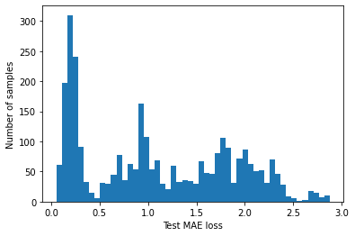
test_mae_loss = np.mean(np.abs(X_test_pred - X_test), axis=1)
plt.hist(test_mae_loss, bins=50)
plt.xlabel('Test MAE loss')
plt.ylabel('Number of samples')
plt.show()
test_score_df = pd.DataFrame(test[TIME_STEPS:])
test_score_df['loss'] = test_mae_loss
test_score_df['threshold'] = threshold
test_score_df['anomaly'] = test_score_df['loss'] > test_score_df['threshold']
test_score_df['Close'] = test[TIME_STEPS:]['Close']
plt.figure(figsize=(12,8))
plt.plot(test_score_df['Date'], test_score_df['loss'], label='Test loss')
plt.plot(test_score_df['Date'], test_score_df['threshold'], label='Threshold')
plt.legend()
plt.show()
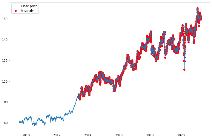
anomalies = test_score_df.loc[test_score_df['anomaly'] == True]
anomalies.shape
(1970, 5)
plt.figure(figsize=(12,8))
plt.plot(test_score_df['Date'], scaler.inverse_transform(test_score_df['Close']),
        label = 'Close price')
plt.scatter(anomalies['Date'], scaler.inverse_transform(anomalies['Close']),
        label = 'Anomaly', c='r')
plt.legend()
plt.show()